Module 1. Neural Networks 01. Image Classification
This is a summary of the CS231n course by Stanford University.
Image Classification
Image Classification is the task of assigning an input imnage one label from a fixed set of categories.
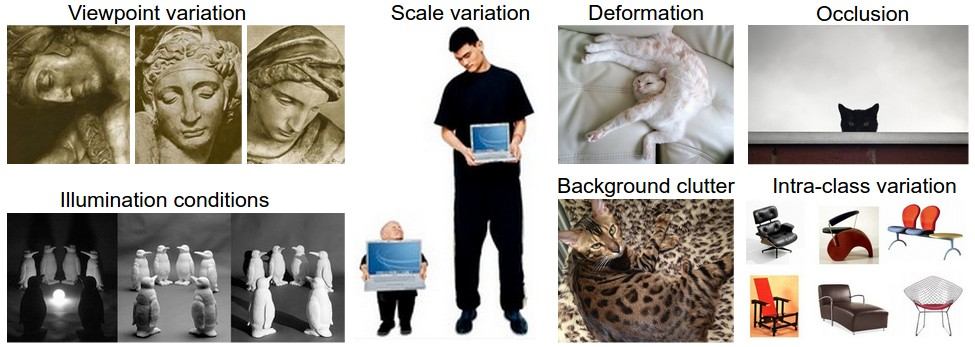
Challenges
- Viewpoint variation: A single instance of an object can be oriented in many ways with respect to the camera.
- Scale variation: Visual classes often exhibit variation in their size (size in the real world, not only in terms of their extent in the image).
- Deformation: Many objects of interest are not rigid bodies and can be deformed in extreme ways.
- Occlusion: The objects of interest can be occluded. Sometimes only a small portion of an object (as little as few pixels) could be visible.
- Illumination conditions: The effects of illumination are drastic on the pixel level.
- Background clutter: The objects of interest may blend into their environment, making them hard to identify.
- Intra-class variation: The classes of interest can often be relatively broad, such as chair. There are many different types of these objects, each with their own appearance.
The image classification pipeline.
Image Classification is to take an array of pixels that represents a single image and assign a label to it.
Nearest Neighbor Classifier
Example image classification dataset: CIFAR-10
One popular toy image classification dataset is the CIFAR-10 dataset. This dataset consists of 60,000 tiny images that are 32 pixels high and wide. Each image is labeled with one of 10 classes. These 60,000 images are partitioned into a training set of 50,000 images and a test set of 10,000 images.
The nearest neighbor classifier will take a test image, compare it to every single one of the training images, and predict the label of the closest training image.
One of the simplest possibilities is to compare the images pixel by pixel and add up all the differences. In other words, given two images and representing them as vectors \(I_1, I_2\) , a reasonable choice for comparing them might be the L1 distance:
\[d_1(I_1, I_2) = \sum_p|I^{p}_{1} - I^{p}_{2}|\]Where the sum is taken over all pixels.
Notice that as an evaluation criterion, it is common to use the accuracy, which measures the fraction of predictions that were correct.
The choice of distance
Another common choice could be to instead use the L2 distance, which has the geometric interpretation of computing the euclidean distance between two vectors.
\[d_2(I_1, I_2) = \sqrt{\sum_p(I^{p}_{1} - I^{p}_{2})^2}\]L1 vs L2
In particular, the L2 distance is much more unforgiving than the L1 distance when it comes to differences between two vectors. That is, the L2 distance prefers many medium disagreements to one big one.
k - Nearest Neighbor Classifier
The idea is very simple: instead of finding the single closest image in the training set, we will find the top k closest images, and have them vote on the label of the test image. Intuitively, higher values of k have a smoothing effect that makes the classifier more resistant to outliers. But what value of k should you use?
Validation sets for Hyperparameter tuning
Hyperparameters and they come up very often in the design of many Machine Learning algorithms that learn from data. It’s often not obvious what values/settings one should choose. In particular, we cannot use the test set for the purpose of tweaking hyperparameters. But if you only use the test set once at end, it remains a good proxy for measuring the generalization of your classifier.
Evaluate on the test set only a single time, at the very end.
Split your training set into training set and a validation set. Use validation set to tune all hyperparameters. At the end run a single time on the test set and report performance.
Cross-validation
In cases where the size of your training data (and therefore also the validation data) might be small, people sometimes use a more sophisticated technique for hyperparameter tuning called cross-validation. For example, in 5-fold cross-validation, we would split the training data into 5 equal folds, use 4 of them for training, and 1 for validation. We would then iterate over which fold is the validation fold, evaluate the performance, and finally average the performance across the different folds.
In practice
In practice, people prefer to avoid cross-validation in favor of having a single validation split, since cross-validation can be computationally expensive. Typical number of folds you can see in practice would be 3-fold, 5-fold or 10-fold cross-validation.
Pros and Cons of Nearest Neighbor classifier
- Pros: Simple to implement, no training time
- Cons: Very slow at test time, very poor performance for high-dimensional data
Summary
- We introduced the problem of Image Classification, in which we are given a set of images that are all labeled with a single category. We are then asked to predict these categories for a novel set of test images and measure the accuracy of the predictions.
- We introduced a simple classifier called the Nearest Neighbor classifier. We saw that there are multiple hyper-parameters (such as value of k, or the type of distance used to compare examples) that are associated with this classifier and that there was no obvious way of choosing them.
- We saw that the correct way to set these hyperparameters is to split your training data into two: a training set and a fake test set, which we call validation set. We try different hyperparameter values and keep the values that lead to the best performance on the validation set.
- If the lack of training data is a concern, we discussed a procedure called cross-validation, which can help reduce noise in estimating which hyperparameters work best.
- Once the best hyperparameters are found, we fix them and perform a single evaluation on the actual test set.
- We saw that Nearest Neighbor can get us about 40% accuracy on CIFAR-10. It is simple to implement but requires us to store the entire training set and it is expensive to evaluate on a test image.
- Finally, we saw that the use of L1 or L2 distances on raw pixel values is not adequate since the distances correlate more strongly with backgrounds and color distributions of images than with their semantic content.