09. Convolutional Neural Networks: Architectures, Convolution / Pooling Layers

원문: Convolutional Neural Networks: Architectures, Convolution / Pooling Layers — CS231n: Convolutional Neural Networks for Visual Recognition (Stanford University) · © 2015 Andrej Karpathy, MIT License

원문을 문단 단위로 인용하고 그 아래에 한국어 번역을 붙였다. 인용 블록이 원문, 그 아래 문단이 번역이며, 역주 박스와 보충 섹션은 원문에 없는 추가 내용이다.

Table of Contents:

목차는 다음과 같다.

• Architecture Overview
• ConvNet Layers
• Convolutional Layer
• Pooling Layer
• Normalization Layer
• Fully-Connected Layer
• Converting Fully-Connected Layers to Convolutional Layers
• ConvNet Architectures
• Layer Patterns
• Layer Sizing Patterns
• Case Studies (LeNet / AlexNet / ZFNet / GoogLeNet / VGGNet)
• Computational Considerations
• Additional References

• 구조 훑어보기
• ConvNet을 이루는 층
• 합성곱 층
• Pooling 층
• 정규화 층
• 완전 연결 층
• 완전 연결 층을 합성곱 층으로 바꾸기
• ConvNet 구조
• 층 배치 패턴
• 층 크기 잡기 패턴
• 사례 연구 (LeNet / AlexNet / ZFNet / GoogLeNet / VGGNet)
• 계산상의 고려사항
• 추가 참고 자료

Convolutional Neural Networks (CNNs / ConvNets)

Convolutional Neural Networks are very similar to ordinary Neural Networks from the previous chapter: they are made up of neurons that have learnable weights and biases. Each neuron receives some inputs, performs a dot product and optionally follows it with a non-linearity. The whole network still expresses a single differentiable score function: from the raw image pixels on one end to class scores at the other. And they still have a loss function (e.g. SVM/Softmax) on the last (fully-connected) layer and all the tips/tricks we developed for learning regular Neural Networks still apply.

합성곱 신경망은 앞 장에서 본 보통의 신경망과 아주 비슷하다. 학습 가능한 가중치와 편향을 가진 뉴런들로 이루어져 있다는 점이 같다. 뉴런 하나하나는 입력을 받아 내적을 계산하고, 필요하면 그 뒤에 비선형성을 씌운다. 신경망 전체는 여전히 미분 가능한 점수 함수 하나를 나타낸다. 한쪽 끝의 날것 그대로의 이미지 픽셀에서 반대쪽 끝의 클래스 점수까지 이어지는 함수다. 마지막 (완전 연결) 층에는 여전히 손실 함수(예컨대 SVM이나 Softmax)가 놓이고, 보통의 신경망을 학습시키려고 다듬어온 요령과 기법도 그대로 적용된다.

So what changes? ConvNet architectures make the explicit assumption that the inputs are images, which allows us to encode certain properties into the architecture. These then make the forward function more efficient to implement and vastly reduce the amount of parameters in the network.

그렇다면 무엇이 달라지는가? ConvNet 구조는 입력이 이미지라고 대놓고 가정한다. 그 덕분에 몇 가지 성질을 구조 자체에 새겨 넣을 수 있다. 그렇게 새겨 넣은 성질은 순전파 함수를 더 효율적으로 구현하게 해주고, 신경망의 매개변수 개수를 크게 줄여준다.

Architecture Overview

Recall: Regular Neural Nets. As we saw in the previous chapter, Neural Networks receive an input (a single vector), and transform it through a series of hidden layers. Each hidden layer is made up of a set of neurons, where each neuron is fully connected to all neurons in the previous layer, and where neurons in a single layer function completely independently and do not share any connections. The last fully-connected layer is called the “output layer” and in classification settings it represents the class scores.

복습: 보통의 신경망. 앞 장에서 봤듯이 신경망은 입력(벡터 하나)을 받아 여러 개의 은닉층을 거치며 변환한다. 은닉층은 저마다 뉴런의 집합으로 이루어지고, 각 뉴런은 앞 층의 모든 뉴런과 완전히 연결된다. 같은 층 안의 뉴런들은 서로 완전히 독립적으로 동작하며 어떤 연결도 공유하지 않는다. 마지막 완전 연결 층은 “출력층”이라 부르고, 분류 문제에서는 클래스 점수를 나타낸다.

Regular Neural Nets don’t scale well to full images. In CIFAR-10, images are only of size 32x32x3 (32 wide, 32 high, 3 color channels), so a single fully-connected neuron in a first hidden layer of a regular Neural Network would have 32*32*3 = 3072 weights. This amount still seems manageable, but clearly this fully-connected structure does not scale to larger images. For example, an image of more respectable size, e.g. 200x200x3, would lead to neurons that have 200*200*3 = 120,000 weights. Moreover, we would almost certainly want to have several such neurons, so the parameters would add up quickly! Clearly, this full connectivity is wasteful and the huge number of parameters would quickly lead to overfitting.

보통의 신경망은 이미지 전체로는 잘 확장되지 않는다. CIFAR-10의 이미지는 크기가 32x32x3(가로 32, 세로 32, 색 채널 3개)밖에 되지 않으므로, 보통의 신경망 첫 은닉층에 있는 완전 연결 뉴런 하나는 32*32*3 = 3072개의 가중치를 갖는다. 이 정도는 아직 감당할 만해 보인다. 하지만 이 완전 연결 구조가 더 큰 이미지로는 확장되지 않는다는 것은 분명하다. 예컨대 200x200x3처럼 좀 더 그럴듯한 크기의 이미지라면 뉴런 하나가 200*200*3 = 120,000개의 가중치를 갖게 된다. 게다가 그런 뉴런을 여러 개 두고 싶을 것이 거의 확실하니 매개변수는 순식간에 불어난다! 이런 완전 연결은 명백히 낭비이고, 어마어마한 매개변수 개수는 금세 과적합으로 이어진다.

3D volumes of neurons. Convolutional Neural Networks take advantage of the fact that the input consists of images and they constrain the architecture in a more sensible way. In particular, unlike a regular Neural Network, the layers of a ConvNet have neurons arranged in 3 dimensions: width, height, depth. (Note that the word depth here refers to the third dimension of an activation volume, not to the depth of a full Neural Network, which can refer to the total number of layers in a network.) For example, the input images in CIFAR-10 are an input volume of activations, and the volume has dimensions 32x32x3 (width, height, depth respectively). As we will soon see, the neurons in a layer will only be connected to a small region of the layer before it, instead of all of the neurons in a fully-connected manner. Moreover, the final output layer would for CIFAR-10 have dimensions 1x1x10, because by the end of the ConvNet architecture we will reduce the full image into a single vector of class scores, arranged along the depth dimension. Here is a visualization:

뉴런을 3차원 부피로 놓는다. 합성곱 신경망은 입력이 이미지라는 사실을 활용해 구조에 더 합리적인 제약을 건다. 특히 보통의 신경망과 달리 ConvNet의 층은 뉴런을 가로, 세로, 깊이의 3차원으로 배열한다. (여기서 깊이라는 말은 활성값 부피(volume)의 세 번째 차원을 가리키며, 신경망 전체의 층 수를 뜻하는 신경망의 깊이와는 다르다.) 예컨대 CIFAR-10의 입력 이미지는 활성값 부피 하나이고, 그 부피의 크기는 32x32x3(각각 가로, 세로, 깊이)이다. 곧 보겠지만 한 층의 뉴런은 앞 층의 모든 뉴런에 완전 연결되는 대신 앞 층의 작은 영역에만 연결된다. 또한 CIFAR-10이라면 마지막 출력층의 크기는 1x1x10이 된다. ConvNet 구조의 끝에 이르면 이미지 전체가 깊이 방향으로 늘어선 클래스 점수 벡터 하나로 줄어들기 때문이다. 그림으로 보면 다음과 같다.

역주. ‘깊이’가 두 가지를 가리킨다는 원문의 경고는 생각보다 자주 걸린다. 활성값 부피의 깊이는 그 부피의 세 번째 차원이다. 입력 이미지에서는 색 채널 수 3이고, CONV 층의 출력에서는 그 층이 쓴 필터의 개수다. 반면 “깊은 신경망”이라고 할 때의 깊이는 층의 개수다. 아래에서 CONV 층의 하이퍼파라미터로 ‘깊이’가 나오면 그것은 언제나 앞쪽, 곧 출력 부피의 세 번째 차원이자 필터 개수를 뜻한다.

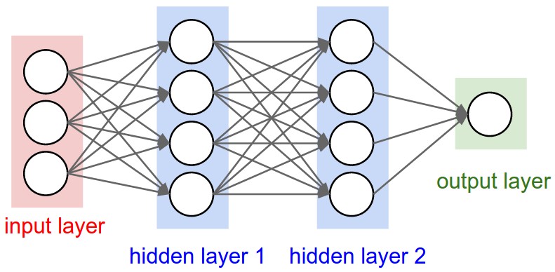
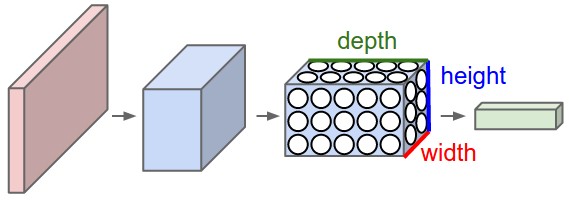Left: A regular 3-layer Neural Network. Right: A ConvNet arranges its neurons in three dimensions (width, height, depth), as visualized in one of the layers. Every layer of a ConvNet transforms the 3D input volume to a 3D output volume of neuron activations. In this example, the red input layer holds the image, so its width and height would be the dimensions of the image, and the depth would be 3 (Red, Green, Blue channels).

왼쪽: 보통의 3층 신경망. 오른쪽: ConvNet은 뉴런을 3차원(가로, 세로, 깊이)으로 배열하며, 그림에서는 그중 한 층을 그렸다. ConvNet의 모든 층은 3차원 입력 부피를 뉴런 활성값의 3차원 출력 부피로 변환한다. 이 예에서 빨간 입력층은 이미지를 담고 있으므로 가로와 세로는 이미지의 크기이고 깊이는 3(빨강, 초록, 파랑 채널)이다.

A ConvNet is made up of Layers. Every Layer has a simple API: It transforms an input 3D volume to an output 3D volume with some differentiable function that may or may not have parameters.

ConvNet은 층으로 이루어진다. 모든 층은 간단한 API 하나를 갖는다. 매개변수가 있을 수도 없을 수도 있는 미분 가능한 함수로 3차원 입력 부피를 3차원 출력 부피로 바꾼다.

Layers used to build ConvNets

As we described above, a simple ConvNet is a sequence of layers, and every layer of a ConvNet transforms one volume of activations to another through a differentiable function. We use three main types of layers to build ConvNet architectures: Convolutional Layer, Pooling Layer, and Fully-Connected Layer (exactly as seen in regular Neural Networks). We will stack these layers to form a full ConvNet architecture.

위에서 설명했듯이 간단한 ConvNet은 층을 죽 늘어놓은 것이고, ConvNet의 각 층은 미분 가능한 함수를 통해 활성값 부피 하나를 다른 활성값 부피로 변환한다. ConvNet 구조를 짜는 데는 주로 세 가지 층을 쓴다. 합성곱 층(Convolutional Layer), pooling 층, 그리고 (보통의 신경망에서 본 것과 똑같은) 완전 연결 층이다. 이 층들을 쌓아 하나의 완전한 ConvNet 구조를 만든다.

Example Architecture: Overview. We will go into more details below, but a simple ConvNet for CIFAR-10 classification could have the architecture [INPUT - CONV - RELU - POOL - FC]. In more detail:

예시 구조 훑어보기. 자세한 내용은 아래에서 다루겠지만, CIFAR-10 분류를 위한 간단한 ConvNet은 [INPUT - CONV - RELU - POOL - FC] 구조를 가질 수 있다. 좀 더 자세히 보면 다음과 같다.

• INPUT [32x32x3] will hold the raw pixel values of the image, in this case an image of width 32, height 32, and with three color channels R,G,B.
• CONV layer will compute the output of neurons that are connected to local regions in the input, each computing a dot product between their weights and a small region they are connected to in the input volume. This may result in volume such as [32x32x12] if we decided to use 12 filters.
• RELU layer will apply an elementwise activation function, such as the \(max(0,x)\) thresholding at zero. This leaves the size of the volume unchanged ([32x32x12]).
• POOL layer will perform a downsampling operation along the spatial dimensions (width, height), resulting in volume such as [16x16x12].
• FC (i.e. fully-connected) layer will compute the class scores, resulting in volume of size [1x1x10], where each of the 10 numbers correspond to a class score, such as among the 10 categories of CIFAR-10. As with ordinary Neural Networks and as the name implies, each neuron in this layer will be connected to all the numbers in the previous volume.

• INPUT [32x32x3]은 이미지의 날것 그대로의 픽셀 값을 담는다. 여기서는 가로 32, 세로 32이고 색 채널이 R, G, B 세 개인 이미지다.
• CONV 층은 입력의 국소 영역에 연결된 뉴런들의 출력을 계산한다. 뉴런마다 자기 가중치와, 입력 부피에서 자기가 연결된 작은 영역 사이의 내적을 계산한다. 필터를 12개 쓰기로 했다면 결과는 [32x32x12] 같은 부피가 된다.
• RELU 층은 \(max(0,x)\)처럼 0에서 자르는 활성화 함수를 원소별로 적용한다. 부피의 크기는 그대로다([32x32x12]).
• POOL 층은 공간 차원(가로, 세로)을 따라 다운샘플링을 수행해 [16x16x12] 같은 부피를 만든다.
• FC(곧 완전 연결) 층은 클래스 점수를 계산해 [1x1x10] 크기의 부피를 만든다. 이 10개의 수는 각각 하나의 클래스 점수에 해당하며, CIFAR-10이라면 10개 범주의 점수다. 보통의 신경망에서와 같고 이름 그대로, 이 층의 각 뉴런은 앞 부피의 모든 수에 연결된다.

In this way, ConvNets transform the original image layer by layer from the original pixel values to the final class scores. Note that some layers contain parameters and other don’t. In particular, the CONV/FC layers perform transformations that are a function of not only the activations in the input volume, but also of the parameters (the weights and biases of the neurons). On the other hand, the RELU/POOL layers will implement a fixed function. The parameters in the CONV/FC layers will be trained with gradient descent so that the class scores that the ConvNet computes are consistent with the labels in the training set for each image.

이런 식으로 ConvNet은 원래 이미지를 층에서 층으로 변환해가며 처음의 픽셀 값에서 최종 클래스 점수까지 데려간다. 어떤 층은 매개변수를 갖고 어떤 층은 갖지 않는다는 점에 유의하자. 특히 CONV/FC 층은 입력 부피의 활성값뿐 아니라 매개변수(뉴런의 가중치와 편향)에도 의존하는 변환을 수행한다. 반면 RELU/POOL 층은 고정된 함수를 구현한다. CONV/FC 층의 매개변수는 경사 하강법으로 학습되어, ConvNet이 계산하는 클래스 점수가 학습 집합의 각 이미지에 붙은 레이블과 맞아떨어지게 된다.

In summary:

정리하면 다음과 같다.

• A ConvNet architecture is in the simplest case a list of Layers that transform the image volume into an output volume (e.g. holding the class scores)
• There are a few distinct types of Layers (e.g. CONV/FC/RELU/POOL are by far the most popular)
• Each Layer accepts an input 3D volume and transforms it to an output 3D volume through a differentiable function
• Each Layer may or may not have parameters (e.g. CONV/FC do, RELU/POOL don’t)
• Each Layer may or may not have additional hyperparameters (e.g. CONV/FC/POOL do, RELU doesn’t)

• ConvNet 구조는 가장 단순하게 보면 이미지 부피를 출력 부피(예컨대 클래스 점수를 담은 것)로 변환하는 층들의 목록이다
• 층에는 몇 가지 종류가 있다(예컨대 CONV/FC/RELU/POOL이 압도적으로 많이 쓰인다)
• 각 층은 3차원 입력 부피를 받아 미분 가능한 함수를 통해 3차원 출력 부피로 변환한다
• 각 층은 매개변수를 가질 수도 있고 갖지 않을 수도 있다(예컨대 CONV/FC는 갖고 RELU/POOL은 갖지 않는다)
• 각 층은 하이퍼파라미터를 따로 가질 수도 있고 갖지 않을 수도 있다(예컨대 CONV/FC/POOL은 갖고 RELU는 갖지 않는다)

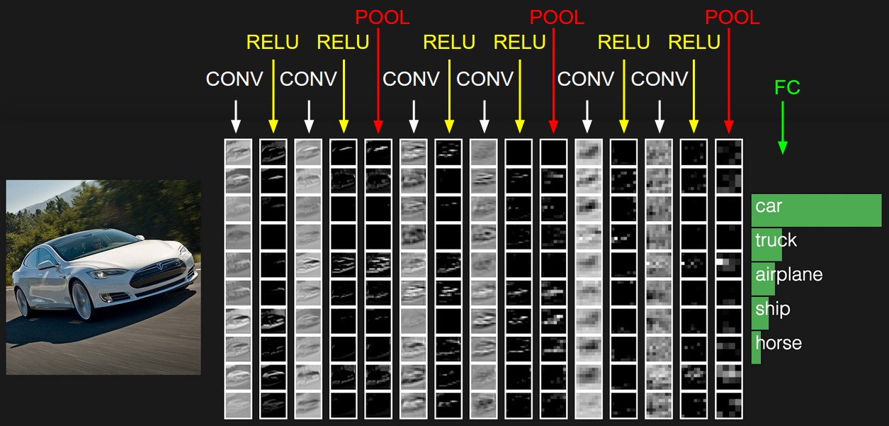The activations of an example ConvNet architecture. The initial volume stores the raw image pixels (left) and the last volume stores the class scores (right). Each volume of activations along the processing path is shown as a column. Since it’s difficult to visualize 3D volumes, we lay out each volume’s slices in rows. The last layer volume holds the scores for each class, but here we only visualize the sorted top 5 scores, and print the labels of each one. The full web-based demo is shown in the header of our website. The architecture shown here is a tiny VGG Net, which we will discuss later.

예시 ConvNet 구조의 활성값. 첫 부피는 날것 그대로의 이미지 픽셀을 담고(왼쪽), 마지막 부피는 클래스 점수를 담는다(오른쪽). 처리 경로를 따라가는 각 활성값 부피를 열 하나로 그렸다. 3차원 부피는 그림으로 나타내기 어려우므로 각 부피의 슬라이스를 행으로 펼쳐 놓았다. 마지막 층의 부피는 클래스마다의 점수를 담고 있지만, 여기서는 정렬해서 상위 5개 점수만 그리고 각각의 레이블을 함께 적었다. 웹 데모 전체는 우리 웹사이트 머리말에서 볼 수 있다. 여기 그린 구조는 작은 VGG Net으로, 뒤에서 다룰 것이다.

We now describe the individual layers and the details of their hyperparameters and their connectivities.

이제 각 층을 하나씩 살펴보며 하이퍼파라미터와 연결 방식을 자세히 설명한다.

Convolutional Layer

The Conv layer is the core building block of a Convolutional Network that does most of the computational heavy lifting.

Conv 층은 합성곱 신경망의 핵심 구성 요소이며, 계산의 무거운 짐을 대부분 짊어진다.

Overview and intuition without brain stuff. Let’s first discuss what the CONV layer computes without brain/neuron analogies. The CONV layer’s parameters consist of a set of learnable filters. Every filter is small spatially (along width and height), but extends through the full depth of the input volume. For example, a typical filter on a first layer of a ConvNet might have size 5x5x3 (i.e. 5 pixels width and height, and 3 because images have depth 3, the color channels). During the forward pass, we slide (more precisely, convolve) each filter across the width and height of the input volume and compute dot products between the entries of the filter and the input at any position. As we slide the filter over the width and height of the input volume we will produce a 2-dimensional activation map that gives the responses of that filter at every spatial position. Intuitively, the network will learn filters that activate when they see some type of visual feature such as an edge of some orientation or a blotch of some color on the first layer, or eventually entire honeycomb or wheel-like patterns on higher layers of the network. Now, we will have an entire set of filters in each CONV layer (e.g. 12 filters), and each of them will produce a separate 2-dimensional activation map. We will stack these activation maps along the depth dimension and produce the output volume.

뇌 이야기 없이 훑어보고 감 잡기. 먼저 뇌나 뉴런에 빗대지 않고 CONV 층이 무엇을 계산하는지 이야기해보자. CONV 층의 매개변수는 학습 가능한 필터의 집합이다. 모든 필터는 공간적으로는(가로와 세로로는) 작지만, 입력 부피의 깊이 전체를 관통한다. 예컨대 ConvNet 첫 층의 전형적인 필터는 크기가 5x5x3일 수 있다(가로세로로 5픽셀이고, 이미지의 깊이가 색 채널 3개이므로 3이다). 순전파 동안 우리는 각 필터를 입력 부피의 가로와 세로를 따라 미끄러뜨리며(더 정확히는 합성곱하며), 필터의 원소들과 그 위치의 입력 사이의 내적을 계산한다. 필터를 입력 부피의 가로와 세로를 따라 미끄러뜨리고 나면, 그 필터가 모든 공간 위치에서 얼마나 반응했는지를 담은 2차원 활성값 지도(activation map)가 만들어진다. 직관적으로 보면 신경망은 어떤 시각적 특징을 봤을 때 활성화되는 필터를 학습하게 된다. 첫 층에서는 어떤 방향의 경계선이나 어떤 색깔의 얼룩 같은 것이고, 더 위쪽 층에 가면 벌집이나 바퀴 모양 전체 같은 것이다. 그런데 CONV 층마다 필터가 통째로 한 벌(예컨대 12개) 있고, 각각이 별개의 2차원 활성값 지도를 만들어낸다. 이 활성값 지도들을 깊이 방향으로 쌓아 출력 부피를 만든다.

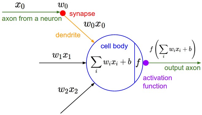
The brain view. If you’re a fan of the brain/neuron analogies, every entry in the 3D output volume can also be interpreted as an output of a neuron that looks at only a small region in the input and shares parameters with all neurons to the left and right spatially (since these numbers all result from applying the same filter).

뇌의 관점. 뇌나 뉴런에 빗대는 것을 좋아한다면, 3차원 출력 부피의 각 원소를 뉴런 하나의 출력으로 해석해도 된다. 그 뉴런은 입력의 작은 영역만 들여다보고, 공간적으로 좌우에 있는 모든 뉴런과 매개변수를 공유한다(이 수들은 모두 같은 필터를 적용해 나온 것이기 때문이다).

We now discuss the details of the neuron connectivities, their arrangement in space, and their parameter sharing scheme.

이제 뉴런의 연결 방식, 공간상의 배치, 매개변수 공유 방식을 차례로 자세히 살펴본다.

Local Connectivity. When dealing with high-dimensional inputs such as images, as we saw above it is impractical to connect neurons to all neurons in the previous volume. Instead, we will connect each neuron to only a local region of the input volume. The spatial extent of this connectivity is a hyperparameter called the receptive field of the neuron (equivalently this is the filter size). The extent of the connectivity along the depth axis is always equal to the depth of the input volume. It is important to emphasize again this asymmetry in how we treat the spatial dimensions (width and height) and the depth dimension: The connections are local in 2D space (along width and height), but always full along the entire depth of the input volume.

국소 연결(local connectivity). 이미지처럼 차원이 높은 입력을 다룰 때는 위에서 봤듯이 앞 부피의 모든 뉴런에 뉴런을 연결하는 것이 현실적이지 않다. 대신 각 뉴런을 입력 부피의 국소 영역에만 연결한다. 이 연결이 공간적으로 뻗는 범위는 하이퍼파라미터이며 그 뉴런의 수용 영역(receptive field)이라 부른다(같은 말로 필터 크기다). 깊이 축을 따라 뻗는 범위는 언제나 입력 부피의 깊이와 같다. 공간 차원(가로와 세로)과 깊이 차원을 이렇게 다르게 다룬다는 비대칭성은 다시 한번 강조해둘 만하다. 연결은 2차원 공간에서는(가로와 세로로는) 국소적이지만, 입력 부피의 깊이 전체로는 언제나 빠짐없이 이어진다.

Example 1. For example, suppose that the input volume has size [32x32x3], (e.g. an RGB CIFAR-10 image). If the receptive field (or the filter size) is 5x5, then each neuron in the Conv Layer will have weights to a [5x5x3] region in the input volume, for a total of 5*5*3 = 75 weights (and +1 bias parameter). Notice that the extent of the connectivity along the depth axis must be 3, since this is the depth of the input volume.

예 1. 예컨대 입력 부피의 크기가 [32x32x3] (예컨대 RGB CIFAR-10 이미지)이라고 하자. 수용 영역(곧 필터 크기)이 5x5라면 Conv 층의 각 뉴런은 입력 부피의 [5x5x3] 영역에 대한 가중치를 갖고, 모두 합쳐 5*5*3 = 75개의 가중치(그리고 편향 매개변수 +1개)를 갖는다. 깊이 축을 따라 뻗는 범위는 반드시 3이어야 하는데, 그것이 입력 부피의 깊이이기 때문이다.

Example 2. Suppose an input volume had size [16x16x20]. Then using an example receptive field size of 3x3, every neuron in the Conv Layer would now have a total of 3*3*20 = 180 connections to the input volume. Notice that, again, the connectivity is local in 2D space (e.g. 3x3), but full along the input depth (20).

예 2. 입력 부피의 크기가 [16x16x20]이라고 하자. 수용 영역 크기를 3x3으로 잡으면 이제 Conv 층의 각 뉴런은 입력 부피에 대해 모두 3*3*20 = 180개의 연결을 갖는다. 여기서도 연결은 2차원 공간에서는 국소적이지만(예컨대 3x3), 입력 깊이(20) 전체로는 빠짐없이 이어진다는 점에 유의하자.

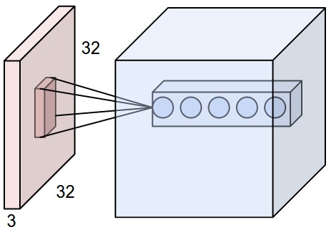
Left: An example input volume in red (e.g. a 32x32x3 CIFAR-10 image), and an example volume of neurons in the first Convolutional layer. Each neuron in the convolutional layer is connected only to a local region in the input volume spatially, but to the full depth (i.e. all color channels). Note, there are multiple neurons (5 in this example) along the depth, all looking at the same region in the input: the lines that connect this column of 5 neurons do not represent the weights (i.e. these 5 neurons do not share the same weights, but they are associated with 5 different filters), they just indicate that these neurons are connected to or looking at the same receptive field or region of the input volume, i.e. they share the same receptive field but not the same weights. Right: The neurons from the Neural Network chapter remain unchanged: They still compute a dot product of their weights with the input followed by a non-linearity, but their connectivity is now restricted to be local spatially.

왼쪽: 빨간색으로 그린 예시 입력 부피(예컨대 32x32x3 CIFAR-10 이미지)와, 첫 합성곱 층의 예시 뉴런 부피. 합성곱 층의 각 뉴런은 입력 부피에서 공간적으로 국소적인 영역에만 연결되지만 깊이로는 전체(곧 모든 색 채널)에 연결된다. 깊이를 따라 여러 개의 뉴런(이 예에서는 5개)이 있고 그것들이 모두 입력의 같은 영역을 들여다본다는 점에 유의하자. 이 5개 뉴런의 기둥을 잇는 선은 가중치를 나타내는 것이 아니다(곧 이 5개 뉴런은 같은 가중치를 공유하지 않으며 서로 다른 5개의 필터에 대응한다). 그 선은 이 뉴런들이 입력 부피의 같은 수용 영역, 곧 같은 영역에 연결되어 있고 그곳을 들여다보고 있다는 것만 나타낸다. 다시 말해 수용 영역은 공유하지만 가중치는 공유하지 않는다. 오른쪽: 신경망 장에서 본 뉴런은 그대로다. 여전히 자기 가중치와 입력의 내적을 계산하고 그 뒤에 비선형성을 씌운다. 다만 이제 연결이 공간적으로 국소적이도록 제한될 뿐이다.

Spatial arrangement. We have explained the connectivity of each neuron in the Conv Layer to the input volume, but we haven’t yet discussed how many neurons there are in the output volume or how they are arranged. Three hyperparameters control the size of the output volume: the depth, stride and zero-padding. We discuss these next:

공간 배치. Conv 층의 각 뉴런이 입력 부피에 어떻게 연결되는지는 설명했지만, 출력 부피에 뉴런이 몇 개나 있고 어떻게 배열되는지는 아직 이야기하지 않았다. 출력 부피의 크기는 세 개의 하이퍼파라미터가 결정한다. 깊이, stride, 그리고 zero-padding이다. 차례로 살펴보자.

1. First, the depth of the output volume is a hyperparameter: it corresponds to the number of filters we would like to use, each learning to look for something different in the input. For example, if the first Convolutional Layer takes as input the raw image, then different neurons along the depth dimension may activate in presence of various oriented edges, or blobs of color. We will refer to a set of neurons that are all looking at the same region of the input as a depth column (some people also prefer the term fibre).
2. Second, we must specify the stride with which we slide the filter. When the stride is 1 then we move the filters one pixel at a time. When the stride is 2 (or uncommonly 3 or more, though this is rare in practice) then the filters jump 2 pixels at a time as we slide them around. This will produce smaller output volumes spatially.
3. As we will soon see, sometimes it will be convenient to pad the input volume with zeros around the border. The size of this zero-padding is a hyperparameter. The nice feature of zero padding is that it will allow us to control the spatial size of the output volumes (most commonly as we’ll see soon we will use it to exactly preserve the spatial size of the input volume so the input and output width and height are the same).

1. 첫째, 출력 부피의 깊이는 하이퍼파라미터다. 쓰고 싶은 필터의 개수에 해당하며, 필터마다 입력에서 서로 다른 것을 찾도록 학습된다. 예컨대 첫 합성곱 층이 날것 그대로의 이미지를 입력으로 받는다면, 깊이 차원을 따라 늘어선 뉴런들은 저마다 다른 방향의 경계선이나 색 얼룩이 있을 때 활성화될 수 있다. 입력의 같은 영역을 들여다보는 뉴런들의 묶음을 깊이 기둥(depth column)이라 부르겠다(fibre라는 말을 더 좋아하는 사람도 있다).
2. 둘째, 필터를 미끄러뜨릴 stride를 정해야 한다. stride가 1이면 필터를 한 번에 한 픽셀씩 옮긴다. stride가 2(드물게는 3 이상이지만 실제로는 거의 없다)면 필터를 미끄러뜨릴 때 한 번에 두 픽셀씩 건너뛴다. 그러면 공간적으로 더 작은 출력 부피가 만들어진다.
3. 곧 보겠지만, 입력 부피의 테두리에 0을 덧대는 것이 편할 때가 있다. 이 zero-padding의 크기는 하이퍼파라미터다. zero padding의 좋은 점은 출력 부피의 공간 크기를 우리가 조절할 수 있게 해준다는 것이다(곧 보겠지만 가장 흔하게는 입력 부피의 공간 크기를 정확히 보존해 입력과 출력의 가로세로가 같아지도록 쓴다).

We can compute the spatial size of the output volume as a function of the input volume size (\(W\)), the receptive field size of the Conv Layer neurons (\(F\)), the stride with which they are applied (\(S\)), and the amount of zero padding used (\(P\)) on the border. You can convince yourself that the correct formula for calculating how many neurons “fit” is given by \((W - F + 2P)/S + 1\). For example for a 7x7 input and a 3x3 filter with stride 1 and pad 0 we would get a 5x5 output. With stride 2 we would get a 3x3 output. Lets also see one more graphical example:

출력 부피의 공간 크기는 입력 부피의 크기(\(W\)), Conv 층 뉴런의 수용 영역 크기(\(F\)), 뉴런을 적용하는 stride(\(S\)), 테두리에 덧댄 zero padding의 양(\(P\))의 함수로 계산할 수 있다. 뉴런이 몇 개나 “들어맞는지” 세는 올바른 공식이 \((W - F + 2P)/S + 1\)이라는 것은 직접 따져보면 납득할 수 있다. 예컨대 7x7 입력에 3x3 필터를 stride 1, 패딩 0으로 적용하면 5x5 출력이 나온다. stride를 2로 하면 3x3 출력이 나온다. 그림으로 된 예를 하나 더 보자.

역주. \((W - F + 2P)/S + 1\)은 외울 것이 아니라 세어보면 나오는 식이다. 패딩까지 더한 입력의 폭은 \(W + 2P\)다. 필터를 맨 왼쪽에 붙여 놓으면 그것만으로 이미 출력 한 칸이 정해지고, 그때 오른쪽에 남는 자리는 \(W + 2P - F\)칸이다. 필터는 그 위를 \(S\)칸씩 건너뛰며 옮겨 가므로 \((W + 2P - F)/S\)번 더 옮길 수 있다. 처음의 한 칸에 옮긴 횟수를 더한 것이 곧 출력 크기이며, 식의 \(+ 1\)이 그 처음 한 칸이다.

그래서 \(W + 2P - F\)가 \(S\)로 나누어떨어지지 않으면 마지막 걸음이 입력 밖으로 삐져나간다. 원문이 곧이어 드는 \(W = 10, F = 3, P = 0, S = 2\)의 예에서 4.5가 나오는 것이 그 경우다. 층 크기를 직접 잡을 때 이 나눗셈이 딱 떨어지는지부터 확인하면, 구조가 맞물리지 않아 생기는 사고의 대부분을 미리 막을 수 있다.

Illustration of spatial arrangement. In this example there is only one spatial dimension (x-axis), one neuron with a receptive field size of F = 3, the input size is W = 5, and there is zero padding of P = 1. Left: The neuron strided across the input in stride of S = 1, giving output of size (5 - 3 + 2)/1+1 = 5. Right: The neuron uses stride of S = 2, giving output of size (5 - 3 + 2)/2+1 = 3. Notice that stride S = 3 could not be used since it wouldn’t fit neatly across the volume. In terms of the equation, this can be determined since (5 - 3 + 2) = 4 is not divisible by 3. The neuron weights are in this example [1,0,-1] (shown on very right), and its bias is zero. These weights are shared across all yellow neurons (see parameter sharing below).

공간 배치를 그림으로 나타낸 것. 이 예에는 공간 차원이 하나(x축)뿐이고 뉴런은 하나이며 수용 영역 크기는 F = 3, 입력 크기는 W = 5, zero padding은 P = 1이다. 왼쪽: 뉴런이 S = 1의 stride로 입력을 훑어 크기 (5 - 3 + 2)/1+1 = 5의 출력을 낸다. 오른쪽: 뉴런이 S = 2의 stride를 써서 크기 (5 - 3 + 2)/2+1 = 3의 출력을 낸다. stride S = 3은 쓸 수 없다는 점에 유의하자. 부피에 딱 맞아떨어지게 들어가지 않기 때문이다. 식으로 보면 (5 - 3 + 2) = 4가 3으로 나누어떨어지지 않는다는 데서 알 수 있다. 이 예에서 뉴런의 가중치는 [1,0,-1]이고(맨 오른쪽에 그려져 있다) 편향은 0이다. 이 가중치는 노란 뉴런 전체가 공유한다(아래의 매개변수 공유 참고).

Use of zero-padding. In the example above on left, note that the input dimension was 5 and the output dimension was equal: also 5. This worked out so because our receptive fields were 3 and we used zero padding of 1. If there was no zero-padding used, then the output volume would have had spatial dimension of only 3, because that is how many neurons would have “fit” across the original input. In general, setting zero padding to be \(P = (F - 1)/2\) when the stride is \(S = 1\) ensures that the input volume and output volume will have the same size spatially. It is very common to use zero-padding in this way and we will discuss the full reasons when we talk more about ConvNet architectures.

zero-padding 쓰기. 위 그림의 왼쪽 예에서 입력 차원이 5였고 출력 차원도 똑같이 5였다는 점을 보자. 이렇게 된 것은 수용 영역이 3이고 zero padding을 1로 썼기 때문이다. zero-padding을 쓰지 않았다면 출력 부피의 공간 차원은 3밖에 되지 않았을 것이다. 원래 입력에 뉴런이 그만큼밖에 “들어맞지” 않기 때문이다. 일반적으로 stride가 \(S = 1\)일 때 zero padding을 \(P = (F - 1)/2\)로 잡으면 입력 부피와 출력 부피의 공간 크기가 같아진다. 이런 식으로 zero-padding을 쓰는 것은 아주 흔하며, 그 이유는 ConvNet 구조를 더 자세히 이야기할 때 온전히 다루겠다.

Constraints on strides. Note again that the spatial arrangement hyperparameters have mutual constraints. For example, when the input has size \(W = 10\), no zero-padding is used \(P = 0\), and the filter size is \(F = 3\), then it would be impossible to use stride \(S = 2\), since \((W - F + 2P)/S + 1 = (10 - 3 + 0) / 2 + 1 = 4.5\), i.e. not an integer, indicating that the neurons don’t “fit” neatly and symmetrically across the input. Therefore, this setting of the hyperparameters is considered to be invalid, and a ConvNet library could throw an exception or zero pad the rest to make it fit, or crop the input to make it fit, or something. As we will see in the ConvNet architectures section, sizing the ConvNets appropriately so that all the dimensions “work out” can be a real headache, which the use of zero-padding and some design guidelines will significantly alleviate.

stride에 걸리는 제약. 공간 배치 하이퍼파라미터들이 서로 제약을 건다는 점을 다시 짚어두자. 예컨대 입력 크기가 \(W = 10\)이고 zero-padding을 쓰지 않아 \(P = 0\)이며 필터 크기가 \(F = 3\)이라면, stride \(S = 2\)는 쓸 수 없다. \((W - F + 2P)/S + 1 = (10 - 3 + 0) / 2 + 1 = 4.5\)로 정수가 아니고, 이는 뉴런이 입력 전체에 깔끔하고 대칭적으로 “들어맞지” 않는다는 뜻이기 때문이다. 따라서 이런 하이퍼파라미터 설정은 유효하지 않은 것으로 본다. ConvNet 라이브러리는 예외를 던지거나, 남는 자리를 0으로 덧대 맞추거나, 입력을 잘라내 맞추는 등의 대응을 할 수 있다. ConvNet 구조를 다루는 절에서 보겠지만 모든 차원이 “맞아떨어지도록” ConvNet의 크기를 잡는 일은 상당한 골칫거리가 될 수 있는데, zero-padding과 몇 가지 설계 지침이 그 부담을 크게 덜어준다.

Real-world example. The Krizhevsky et al. architecture that won the ImageNet challenge in 2012 accepted images of size [227x227x3]. On the first Convolutional Layer, it used neurons with receptive field size \(F = 11\), stride \(S = 4\) and no zero padding \(P = 0\). Since (227 - 11)/4 + 1 = 55, and since the Conv layer had a depth of \(K = 96\), the Conv layer output volume had size [55x55x96]. Each of the 55*55*96 neurons in this volume was connected to a region of size [11x11x3] in the input volume. Moreover, all 96 neurons in each depth column are connected to the same [11x11x3] region of the input, but of course with different weights. As a fun aside, if you read the actual paper it claims that the input images were 224x224, which is surely incorrect because (224 - 11)/4 + 1 is quite clearly not an integer. This has confused many people in the history of ConvNets and little is known about what happened. My own best guess is that Alex used zero-padding of 3 extra pixels that he does not mention in the paper.

실제 사례. 2012년 ImageNet 챌린지에서 우승한 Krizhevsky et al. 구조는 [227x227x3] 크기의 이미지를 받았다. 첫 합성곱 층에서는 수용 영역 크기 \(F = 11\), stride \(S = 4\), zero padding 없이 \(P = 0\)인 뉴런을 썼다. (227 - 11)/4 + 1 = 55이고 Conv 층의 깊이가 \(K = 96\)이었으므로 Conv 층 출력 부피의 크기는 [55x55x96]이었다. 이 부피에 있는 55*55*96개의 뉴런은 각각 입력 부피의 [11x11x3] 크기 영역에 연결되었다. 또한 각 깊이 기둥의 96개 뉴런은 모두 입력의 같은 [11x11x3] 영역에 연결되지만 물론 가중치는 서로 다르다. 재미있는 곁가지로, 실제 논문을 읽어보면 입력 이미지가 224x224였다고 되어 있는데 이는 틀린 것이 분명하다. (224 - 11)/4 + 1이 정수가 아니라는 것은 누가 봐도 명백하기 때문이다. 이 대목은 ConvNet의 역사에서 많은 사람을 헷갈리게 했고 무슨 일이 있었는지는 알려진 바가 거의 없다. 내 나름의 추측으로는 Alex가 논문에 적지 않은 3픽셀짜리 zero-padding을 더 썼을 것 같다.

Parameter Sharing. Parameter sharing scheme is used in Convolutional Layers to control the number of parameters. Using the real-world example above, we see that there are 55*55*96 = 290,400 neurons in the first Conv Layer, and each has 11*11*3 = 363 weights and 1 bias. Together, this adds up to 290400 * 364 = 105,705,600 parameters on the first layer of the ConvNet alone. Clearly, this number is very high.

매개변수 공유. 합성곱 층에서는 매개변수 개수를 억누르기 위해 매개변수 공유 방식을 쓴다. 위의 실제 사례를 보면 첫 Conv 층에 55*55*96 = 290,400개의 뉴런이 있고, 뉴런마다 11*11*3 = 363개의 가중치와 편향 1개를 갖는다. 다 합치면 ConvNet의 첫 층 하나에서만 290400 * 364 = 105,705,600개의 매개변수가 된다. 이 수가 아주 크다는 것은 분명하다.

It turns out that we can dramatically reduce the number of parameters by making one reasonable assumption: That if one feature is useful to compute at some spatial position (x,y), then it should also be useful to compute at a different position (x2,y2). In other words, denoting a single 2-dimensional slice of depth as a depth slice (e.g. a volume of size [55x55x96] has 96 depth slices, each of size [55x55]), we are going to constrain the neurons in each depth slice to use the same weights and bias. With this parameter sharing scheme, the first Conv Layer in our example would now have only 96 unique set of weights (one for each depth slice), for a total of 96*11*11*3 = 34,848 unique weights, or 34,944 parameters (+96 biases). Alternatively, all 55*55 neurons in each depth slice will now be using the same parameters. In practice during backpropagation, every neuron in the volume will compute the gradient for its weights, but these gradients will be added up across each depth slice and only update a single set of weights per slice.

그런데 그럴듯한 가정 하나를 세우면 매개변수 개수를 극적으로 줄일 수 있다. 어떤 특징을 공간상의 위치 (x,y)에서 계산하는 것이 유용하다면 다른 위치 (x2,y2)에서 계산하는 것도 유용하리라는 가정이다. 달리 말해, 깊이 방향으로 잘라낸 2차원 조각 하나를 깊이 슬라이스(depth slice)라 부르기로 하면(예컨대 [55x55x96] 크기의 부피에는 각각 [55x55]인 깊이 슬라이스가 96개 있다), 각 깊이 슬라이스 안의 뉴런들이 같은 가중치와 편향을 쓰도록 제약을 건다는 뜻이다. 이 매개변수 공유 방식을 쓰면 우리 예의 첫 Conv 층은 이제 (깊이 슬라이스마다 하나씩) 96벌의 고유한 가중치만 갖게 되어, 고유한 가중치가 모두 96*11*11*3 = 34,848개, 매개변수로는 34,944개(편향 96개를 더해)가 된다. 달리 보면 각 깊이 슬라이스의 55*55개 뉴런이 모두 같은 매개변수를 쓰게 되는 것이다. 실제 역전파에서는 부피의 모든 뉴런이 자기 가중치에 대한 기울기를 계산하지만, 이 기울기들은 깊이 슬라이스별로 모두 더해져 슬라이스마다 가중치 한 벌만 갱신한다.

Notice that if all neurons in a single depth slice are using the same weight vector, then the forward pass of the CONV layer can in each depth slice be computed as a convolution of the neuron’s weights with the input volume (Hence the name: Convolutional Layer). This is why it is common to refer to the sets of weights as a filter (or a kernel), that is convolved with the input.

한 깊이 슬라이스의 모든 뉴런이 같은 가중치 벡터를 쓴다면, CONV 층의 순전파는 깊이 슬라이스마다 그 뉴런의 가중치와 입력 부피의 합성곱(convolution)으로 계산할 수 있다는 점에 유의하자(합성곱 층이라는 이름이 여기서 나왔다). 그래서 이 가중치 한 벌을 입력과 합성곱되는 필터(filter) 또는 커널(kernel)이라 부르는 것이 흔하다.

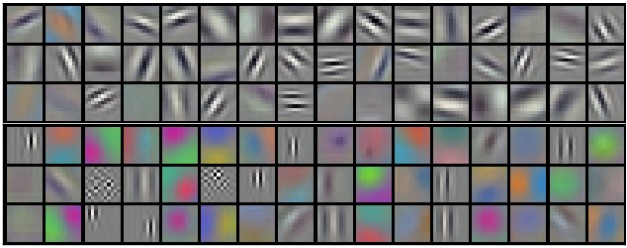Example filters learned by Krizhevsky et al. Each of the 96 filters shown here is of size [11x11x3], and each one is shared by the 55*55 neurons in one depth slice. Notice that the parameter sharing assumption is relatively reasonable: If detecting a horizontal edge is important at some location in the image, it should intuitively be useful at some other location as well due to the translationally-invariant structure of images. There is therefore no need to relearn to detect a horizontal edge at every one of the 55*55 distinct locations in the Conv layer output volume.

Krizhevsky et al.이 학습시킨 필터의 예. 여기 그린 96개 필터는 각각 [11x11x3] 크기이며, 하나하나가 깊이 슬라이스 하나 안의 55*55개 뉴런에 공유된다. 매개변수 공유 가정이 비교적 합리적이라는 점에 유의하자. 이미지의 어떤 위치에서 가로 경계선을 찾아내는 것이 중요하다면, 이미지는 평행이동에 대해 구조가 변하지 않으므로 다른 위치에서도 직관적으로 그것이 유용할 것이다. 따라서 Conv 층 출력 부피의 55*55개 위치마다 가로 경계선 찾는 법을 새로 배울 필요가 없다.

Note that sometimes the parameter sharing assumption may not make sense. This is especially the case when the input images to a ConvNet have some specific centered structure, where we should expect, for example, that completely different features should be learned on one side of the image than another. One practical example is when the input are faces that have been centered in the image. You might expect that different eye-specific or hair-specific features could (and should) be learned in different spatial locations. In that case it is common to relax the parameter sharing scheme, and instead simply call the layer a Locally-Connected Layer.

매개변수 공유 가정이 말이 되지 않을 때도 있다는 점에 유의하자. 특히 ConvNet에 들어가는 입력 이미지가 특정한 구조를 가운데에 맞춰 담고 있을 때가 그렇다. 그런 경우에는 이미지의 한쪽에서 배워야 할 특징이 다른 쪽에서 배워야 할 특징과 완전히 달라지리라고 기대하게 된다. 실제 예로 이미지 가운데에 얼굴을 맞춰 놓은 입력을 들 수 있다. 눈에 관한 특징과 머리카락에 관한 특징이 서로 다른 공간 위치에서 학습될 수 있고 또 그래야 한다고 기대할 만하다. 그런 경우에는 매개변수 공유 방식을 느슨하게 푸는 것이 보통이며, 그렇게 한 층은 그냥 국소 연결 층(Locally-Connected Layer)이라 부른다.

Numpy examples. To make the discussion above more concrete, lets express the same ideas but in code and with a specific example. Suppose that the input volume is a numpy array X. Then:

Numpy 예제. 위의 논의를 좀 더 구체적으로 만들기 위해 같은 내용을 코드와 구체적인 예로 나타내보자. 입력 부피가 numpy 배열 X라고 하자. 그러면 다음과 같다.

• A depth column (or a fibre) at position (x,y) would be the activations X[x,y,:].
• A depth slice, or equivalently an activation map at depth d would be the activations X[:,:,d].

• 위치 (x,y)에서의 깊이 기둥(또는 fibre)은 활성값 X[x,y,:]이다.
• 깊이 d에서의 깊이 슬라이스, 같은 말로 활성값 지도는 활성값 X[:,:,d]이다.

Conv Layer Example. Suppose that the input volume X has shape X.shape: (11,11,4). Suppose further that we use no zero padding (\(P = 0\)), that the filter size is \(F = 5\), and that the stride is \(S = 2\). The output volume would therefore have spatial size (11-5)/2+1 = 4, giving a volume with width and height of 4. The activation map in the output volume (call it V), would then look as follows (only some of the elements are computed in this example):

Conv 층 예제. 입력 부피 X의 모양이 X.shape: (11,11,4)라고 하자. 또 zero padding을 쓰지 않고(\(P = 0\)) 필터 크기가 \(F = 5\)이며 stride가 \(S = 2\)라고 하자. 그러면 출력 부피의 공간 크기는 (11-5)/2+1 = 4가 되어 가로세로가 4인 부피가 나온다. 출력 부피의 활성값 지도(V라고 부르자)는 다음과 같이 생겼다(이 예에서는 일부 원소만 계산해 보인다).

• V[0,0,0] = np.sum(X[:5,:5,:] * W0) + b0
• V[1,0,0] = np.sum(X[2:7,:5,:] * W0) + b0
• V[2,0,0] = np.sum(X[4:9,:5,:] * W0) + b0
• V[3,0,0] = np.sum(X[6:11,:5,:] * W0) + b0

• V[0,0,0] = np.sum(X[:5,:5,:] * W0) + b0
• V[1,0,0] = np.sum(X[2:7,:5,:] * W0) + b0
• V[2,0,0] = np.sum(X[4:9,:5,:] * W0) + b0
• V[3,0,0] = np.sum(X[6:11,:5,:] * W0) + b0

Remember that in numpy, the operation * above denotes elementwise multiplication between the arrays. Notice also that the weight vector W0 is the weight vector of that neuron and b0 is the bias. Here, W0 is assumed to be of shape W0.shape: (5,5,4), since the filter size is 5 and the depth of the input volume is 4. Notice that at each point, we are computing the dot product as seen before in ordinary neural networks. Also, we see that we are using the same weight and bias (due to parameter sharing), and where the dimensions along the width are increasing in steps of 2 (i.e. the stride). To construct a second activation map in the output volume, we would have:

numpy에서 위의 * 연산은 배열 사이의 원소별 곱을 뜻한다는 것을 기억하자. 또 가중치 벡터 W0은 그 뉴런의 가중치 벡터이고 b0은 편향이다. 여기서 W0의 모양은 W0.shape: (5,5,4)라고 가정했다. 필터 크기가 5이고 입력 부피의 깊이가 4이기 때문이다. 각 지점에서 우리가 계산하는 것이 보통의 신경망에서 봤던 그 내적이라는 점에 유의하자. 또한 (매개변수 공유 때문에) 같은 가중치와 편향을 쓰고 있고, 가로 방향의 인덱스가 2씩, 곧 stride만큼 늘어나고 있다는 것도 볼 수 있다. 출력 부피에 두 번째 활성값 지도를 만들려면 다음과 같이 하면 된다.

• V[0,0,1] = np.sum(X[:5,:5,:] * W1) + b1
• V[1,0,1] = np.sum(X[2:7,:5,:] * W1) + b1
• V[2,0,1] = np.sum(X[4:9,:5,:] * W1) + b1
• V[3,0,1] = np.sum(X[6:11,:5,:] * W1) + b1
• V[0,1,1] = np.sum(X[:5,2:7,:] * W1) + b1 (example of going along y)
• V[2,3,1] = np.sum(X[4:9,6:11,:] * W1) + b1 (or along both)

• V[0,0,1] = np.sum(X[:5,:5,:] * W1) + b1
• V[1,0,1] = np.sum(X[2:7,:5,:] * W1) + b1
• V[2,0,1] = np.sum(X[4:9,:5,:] * W1) + b1
• V[3,0,1] = np.sum(X[6:11,:5,:] * W1) + b1
• V[0,1,1] = np.sum(X[:5,2:7,:] * W1) + b1 (y 방향으로 가는 예)
• V[2,3,1] = np.sum(X[4:9,6:11,:] * W1) + b1 (두 방향 모두로 가는 예)

where we see that we are indexing into the second depth dimension in V (at index 1) because we are computing the second activation map, and that a different set of parameters (W1) is now used. In the example above, we are for brevity leaving out some of the other operations the Conv Layer would perform to fill the other parts of the output array V. Additionally, recall that these activation maps are often followed elementwise through an activation function such as ReLU, but this is not shown here.

여기서는 두 번째 활성값 지도를 계산하고 있으므로 V의 깊이 차원을 두 번째 자리(인덱스 1)로 잡고 있고, 이제 다른 매개변수 한 벌(W1)을 쓰고 있다는 것을 볼 수 있다. 위 예에서는 간결하게 쓰려고 Conv 층이 출력 배열 V의 나머지 부분을 채우기 위해 수행할 다른 연산들을 생략했다. 덧붙여, 이 활성값 지도들은 흔히 ReLU 같은 활성화 함수를 원소별로 통과하지만 여기서는 그것도 보이지 않았다.

Summary. To summarize, the Conv Layer:

정리. Conv 층을 정리하면 다음과 같다.

• Accepts a volume of size \(W_1 \times H_1 \times D_1\)
• Requires four hyperparameters:
• Number of filters \(K\),
• their spatial extent \(F\),
• the stride \(S\),
• the amount of zero padding \(P\).
• Produces a volume of size \(W_2 \times H_2 \times D_2\) where:
• \[W_2 = (W_1 - F + 2P)/S + 1\]
• \(H_2 = (H_1 - F + 2P)/S + 1\) (i.e. width and height are computed equally by symmetry)
• \[D_2 = K\]
• With parameter sharing, it introduces \(F \cdot F \cdot D_1\) weights per filter, for a total of \((F \cdot F \cdot D_1) \cdot K\) weights and \(K\) biases.
• In the output volume, the \(d\)-th depth slice (of size \(W_2 \times H_2\)) is the result of performing a valid convolution of the \(d\)-th filter over the input volume with a stride of \(S\), and then offset by \(d\)-th bias.

• 크기 \(W_1 \times H_1 \times D_1\)의 부피를 입력으로 받는다
• 하이퍼파라미터 네 개를 필요로 한다:
• 필터의 개수 \(K\),
• 필터의 공간적 크기 \(F\),
• stride \(S\),
• zero padding의 양 \(P\).
• 크기 \(W_2 \times H_2 \times D_2\)의 부피를 만들어낸다. 여기서:
• \[W_2 = (W_1 - F + 2P)/S + 1\]
• \(H_2 = (H_1 - F + 2P)/S + 1\) (대칭이므로 가로와 세로를 같은 식으로 계산한다)
• \[D_2 = K\]
• 매개변수 공유를 쓰면 필터마다 \(F \cdot F \cdot D_1\)개의 가중치가 생기므로, 모두 합쳐 \((F \cdot F \cdot D_1) \cdot K\)개의 가중치와 \(K\)개의 편향이 생긴다.
• 출력 부피에서 \(d\)번째 깊이 슬라이스(크기 \(W_2 \times H_2\))는 \(d\)번째 필터를 입력 부피 위에서 stride \(S\)로 유효 합성곱한 결과에 \(d\)번째 편향을 더한 것이다.

A common setting of the hyperparameters is \(F = 3, S = 1, P = 1\). However, there are common conventions and rules of thumb that motivate these hyperparameters. See the ConvNet architectures section below.

하이퍼파라미터를 흔히 \(F = 3, S = 1, P = 1\)로 잡는다. 다만 이런 값이 나오게 된 관례와 어림법이 따로 있다. 아래 ConvNet 구조 절을 참고하자.

Convolution Demo. Below is a running demo of a CONV layer. Since 3D volumes are hard to visualize, all the volumes (the input volume (in blue), the weight volumes (in red), the output volume (in green)) are visualized with each depth slice stacked in rows. The input volume is of size \(W_1 = 5, H_1 = 5, D_1 = 3\), and the CONV layer parameters are \(K = 2, F = 3, S = 2, P = 1\). That is, we have two filters of size \(3 \times 3\), and they are applied with a stride of 2. Therefore, the output volume size has spatial size (5 - 3 + 2)/2 + 1 = 3. Moreover, notice that a padding of \(P = 1\) is applied to the input volume, making the outer border of the input volume zero. The visualization below iterates over the output activations (green), and shows that each element is computed by elementwise multiplying the highlighted input (blue) with the filter (red), summing it up, and then offsetting the result by the bias.

합성곱 데모. 아래는 CONV 층이 돌아가는 데모다. 3차원 부피는 그림으로 나타내기 어려우므로 모든 부피(파란색 입력 부피, 빨간색 가중치 부피, 초록색 출력 부피)를 깊이 슬라이스별로 행에 쌓아 그렸다. 입력 부피의 크기는 \(W_1 = 5, H_1 = 5, D_1 = 3\)이고 CONV 층의 매개변수는 \(K = 2, F = 3, S = 2, P = 1\)이다. 곧 \(3 \times 3\) 크기의 필터 두 개를 stride 2로 적용한다. 따라서 출력 부피의 공간 크기는 (5 - 3 + 2)/2 + 1 = 3이 된다. 또한 입력 부피에 \(P = 1\)의 패딩을 적용해 입력 부피의 바깥 테두리를 0으로 만들었다는 점에 유의하자. 아래 시각화는 출력 활성값(초록색)을 하나씩 훑어가면서, 각 원소가 강조된 입력(파란색)과 필터(빨간색)를 원소별로 곱해 더한 뒤 편향만큼 옮겨서 계산된다는 것을 보여준다.

Open the interactive demo on the original cs231n page

위 링크를 누르면 앞 문단이 설명한 \(K = 2, F = 3, S = 2, P = 1\) 설정에서 출력 활성값이 하나씩 계산되는 과정을 움직이는 그림으로 볼 수 있는데, 이 데모 앱은 여기에 옮겨 싣지 않았으므로 원래의 cs231n 페이지에서 열린다.

Implementation as Matrix Multiplication. Note that the convolution operation essentially performs dot products between the filters and local regions of the input. A common implementation pattern of the CONV layer is to take advantage of this fact and formulate the forward pass of a convolutional layer as one big matrix multiply as follows:

행렬 곱으로 구현하기. 합성곱 연산은 본질적으로 필터와 입력의 국소 영역들 사이의 내적을 계산한다는 점에 유의하자. CONV 층을 구현하는 흔한 방식은 이 사실을 이용해 합성곱 층의 순전파를 다음처럼 커다란 행렬 곱 한 번으로 바꿔 쓰는 것이다.

1. The local regions in the input image are stretched out into columns in an operation commonly called im2col. For example, if the input is [227x227x3] and it is to be convolved with 11x11x3 filters at stride 4, then we would take [11x11x3] blocks of pixels in the input and stretch each block into a column vector of size 11*11*3 = 363. Iterating this process in the input at stride of 4 gives (227-11)/4+1 = 55 locations along both width and height, leading to an output matrix X_col of im2col of size [363 x 3025], where every column is a stretched out receptive field and there are 55*55 = 3025 of them in total. Note that since the receptive fields overlap, every number in the input volume may be duplicated in multiple distinct columns.
2. The weights of the CONV layer are similarly stretched out into rows. For example, if there are 96 filters of size [11x11x3] this would give a matrix W_row of size [96 x 363].
3. The result of a convolution is now equivalent to performing one large matrix multiply np.dot(W_row, X_col), which evaluates the dot product between every filter and every receptive field location. In our example, the output of this operation would be [96 x 3025], giving the output of the dot product of each filter at each location.
4. The result must finally be reshaped back to its proper output dimension [55x55x96].

1. 입력 이미지의 국소 영역들을 열로 펴는데, 이 연산을 흔히 im2col이라 부른다. 예컨대 입력이 [227x227x3]이고 11x11x3 필터를 stride 4로 합성곱한다면, 입력에서 [11x11x3] 크기의 픽셀 덩어리를 떼어내 각각 크기 11*11*3 = 363인 열 벡터로 편다. 이 과정을 stride 4로 입력 위에서 반복하면 가로와 세로 양쪽으로 (227-11)/4+1 = 55개의 위치가 나오므로, im2col의 출력 행렬 X_col은 [363 x 3025] 크기가 된다. 각 열은 펼쳐진 수용 영역 하나이고 그런 열이 모두 55*55 = 3025개 있다. 수용 영역들이 서로 겹치므로 입력 부피의 어떤 수는 서로 다른 여러 열에 중복해서 들어갈 수 있다는 점에 유의하자.
2. CONV 층의 가중치도 비슷하게 행으로 편다. 예컨대 [11x11x3] 크기의 필터가 96개라면 [96 x 363] 크기의 행렬 W_row가 나온다.
3. 이제 합성곱의 결과는 커다란 행렬 곱 np.dot(W_row, X_col) 한 번과 같아진다. 이 곱은 모든 필터와 모든 수용 영역 위치 사이의 내적을 계산한다. 우리 예에서 이 연산의 출력은 [96 x 3025]가 되며, 각 필터를 각 위치에 적용한 내적 결과를 담는다.
4. 마지막으로 결과를 원래의 출력 차원 [55x55x96]으로 되돌려 모양을 바꿔야 한다.

This approach has the downside that it can use a lot of memory, since some values in the input volume are replicated multiple times in X_col. However, the benefit is that there are many very efficient implementations of Matrix Multiplication that we can take advantage of (for example, in the commonly used BLAS API). Moreover, the same im2col idea can be reused to perform the pooling operation, which we discuss next.

이 방식은 입력 부피의 어떤 값들이 X_col에 여러 번 복제되므로 메모리를 많이 쓸 수 있다는 단점이 있다. 하지만 행렬 곱은 대단히 효율적인 구현이 많이 나와 있어(예컨대 널리 쓰이는 BLAS API가 있다) 그것을 그대로 가져다 쓸 수 있다는 이점이 있다. 게다가 같은 im2col 아이디어를 다음에 다룰 pooling 연산에도 재사용할 수 있다.

Backpropagation. The backward pass for a convolution operation (for both the data and the weights) is also a convolution (but with spatially-flipped filters). This is easy to derive in the 1-dimensional case with a toy example (not expanded on for now).

역전파. 합성곱 연산의 역방향 진행은 (데이터에 대해서든 가중치에 대해서든) 역시 합성곱이다(다만 필터를 공간적으로 뒤집는다). 1차원의 장난감 예를 가지고 유도해보면 어렵지 않다(여기서는 더 펼치지 않는다).

1x1 convolution. As an aside, several papers use 1x1 convolutions, as first investigated by Network in Network. Some people are at first confused to see 1x1 convolutions especially when they come from signal processing background. Normally signals are 2-dimensional so 1x1 convolutions do not make sense (it’s just pointwise scaling). However, in ConvNets this is not the case because one must remember that we operate over 3-dimensional volumes, and that the filters always extend through the full depth of the input volume. For example, if the input is [32x32x3] then doing 1x1 convolutions would effectively be doing 3-dimensional dot products (since the input depth is 3 channels).

1x1 합성곱. 곁가지로, Network in Network가 처음 파고든 이래 여러 논문이 1x1 합성곱을 쓴다. 신호 처리 쪽에서 온 사람이라면 1x1 합성곱을 보고 처음에는 헷갈리기도 한다. 보통 신호는 2차원이므로 1x1 합성곱은 말이 되지 않기 때문이다(그저 점마다 크기를 조절하는 것일 뿐이다). 하지만 ConvNet에서는 이야기가 다르다. 우리가 3차원 부피 위에서 연산하고 있고 필터는 언제나 입력 부피의 깊이 전체를 관통한다는 것을 기억해야 한다. 예컨대 입력이 [32x32x3]이라면 1x1 합성곱은 사실상 3차원 내적을 하는 셈이다(입력 깊이가 채널 3개이기 때문이다).

Dilated convolutions. A recent development (e.g. see paper by Fisher Yu and Vladlen Koltun) is to introduce one more hyperparameter to the CONV layer called the dilation. So far we’ve only discussed CONV filters that are contiguous. However, it’s possible to have filters that have spaces between each cell, called dilation. As an example, in one dimension a filter w of size 3 would compute over input x the following: w[0]*x[0] + w[1]*x[1] + w[2]*x[2]. This is dilation of 0. For dilation 1 the filter would instead compute w[0]*x[0] + w[1]*x[2] + w[2]*x[4]; In other words there is a gap of 1 between the applications. This can be very useful in some settings to use in conjunction with 0-dilated filters because it allows you to merge spatial information across the inputs much more agressively with fewer layers. For example, if you stack two 3x3 CONV layers on top of each other then you can convince yourself that the neurons on the 2nd layer are a function of a 5x5 patch of the input (we would say that the effective receptive field of these neurons is 5x5). If we use dilated convolutions then this effective receptive field would grow much quicker.

팽창 합성곱. 최근의 진전으로(예컨대 Fisher Yu와 Vladlen Koltun의 논문을 보라) CONV 층에 팽창(dilation)이라는 하이퍼파라미터를 하나 더 도입하는 것이 있다. 지금까지는 칸이 서로 붙어 있는 CONV 필터만 이야기했다. 하지만 칸 사이에 틈이 있는 필터도 가능하고 이것을 팽창이라 부른다. 예를 들어 1차원에서 크기 3인 필터 w는 입력 x에 대해 w[0]*x[0] + w[1]*x[1] + w[2]*x[2]를 계산한다. 이것이 팽창 0이다. 팽창 1이라면 필터는 대신 w[0]*x[0] + w[1]*x[2] + w[2]*x[4]를 계산한다. 다시 말해 적용 지점 사이에 1칸의 틈이 생긴다. 이것을 팽창 0인 필터와 함께 쓰면 어떤 상황에서는 매우 쓸모가 있는데, 더 적은 층으로 입력 전체의 공간 정보를 훨씬 공격적으로 합칠 수 있기 때문이다. 예컨대 3x3 CONV 층 두 개를 위아래로 쌓으면 두 번째 층의 뉴런이 입력의 5x5 조각의 함수라는 것을 직접 따져 확인할 수 있다(이 뉴런들의 실효 수용 영역이 5x5라고 말한다). 팽창 합성곱을 쓰면 이 실효 수용 영역이 훨씬 빠르게 커진다.

Pooling Layer

It is common to periodically insert a Pooling layer in-between successive Conv layers in a ConvNet architecture. Its function is to progressively reduce the spatial size of the representation to reduce the amount of parameters and computation in the network, and hence to also control overfitting. The Pooling Layer operates independently on every depth slice of the input and resizes it spatially, using the MAX operation. The most common form is a pooling layer with filters of size 2x2 applied with a stride of 2 downsamples every depth slice in the input by 2 along both width and height, discarding 75% of the activations. Every MAX operation would in this case be taking a max over 4 numbers (little 2x2 region in some depth slice). The depth dimension remains unchanged. More generally, the pooling layer:

ConvNet 구조에서는 잇달아 놓인 Conv 층 사이사이에 Pooling 층을 주기적으로 끼워 넣는 것이 흔하다. 그 역할은 표현의 공간 크기를 점진적으로 줄여 신경망의 매개변수와 계산량을 줄이고, 그럼으로써 과적합도 억제하는 것이다. Pooling 층은 입력의 깊이 슬라이스마다 독립적으로 동작하며 MAX 연산으로 공간 크기를 줄인다. 가장 흔한 형태는 크기 2x2인 필터를 stride 2로 적용하는 pooling 층으로, 입력의 모든 깊이 슬라이스를 가로세로 양쪽으로 2배씩 다운샘플링해 활성값의 75%를 버린다. 이 경우 MAX 연산 하나하나는 네 개의 수(어떤 깊이 슬라이스의 작은 2x2 영역)에서 최댓값을 고르는 것이 된다. 깊이 차원은 그대로 유지된다. 더 일반적으로 pooling 층은 다음과 같다.

• Accepts a volume of size \(W_1 \times H_1 \times D_1\)
• Requires two hyperparameters:
• their spatial extent \(F\),
• the stride \(S\),
• Produces a volume of size \(W_2 \times H_2 \times D_2\) where:
• \[W_2 = (W_1 - F)/S + 1\]
• \[H_2 = (H_1 - F)/S + 1\]
• \[D_2 = D_1\]
• Introduces zero parameters since it computes a fixed function of the input
• For Pooling layers, it is not common to pad the input using zero-padding.

• 크기 \(W_1 \times H_1 \times D_1\)의 부피를 입력으로 받는다
• 하이퍼파라미터 두 개를 필요로 한다:
• 필터의 공간적 크기 \(F\),
• stride \(S\),
• 크기 \(W_2 \times H_2 \times D_2\)의 부피를 만들어낸다. 여기서:
• \[W_2 = (W_1 - F)/S + 1\]
• \[H_2 = (H_1 - F)/S + 1\]
• \[D_2 = D_1\]
• 입력의 고정된 함수를 계산하므로 매개변수를 하나도 만들지 않는다
• Pooling 층에서는 입력에 zero-padding을 덧대는 것이 흔하지 않다.

It is worth noting that there are only two commonly seen variations of the max pooling layer found in practice: A pooling layer with \(F = 3, S = 2\) (also called overlapping pooling), and more commonly \(F = 2, S = 2\). Pooling sizes with larger receptive fields are too destructive.

실제로 쓰이는 max pooling 층의 변형은 흔히 두 가지뿐이라는 점을 짚어둘 만하다. \(F = 3, S = 2\)인 pooling 층(겹치는 pooling이라고도 한다)과, 더 흔하게는 \(F = 2, S = 2\)인 것이다. 수용 영역이 더 큰 pooling 크기는 정보를 너무 많이 망가뜨린다.

General pooling. In addition to max pooling, the pooling units can also perform other functions, such as average pooling or even L2-norm pooling. Average pooling was often used historically but has recently fallen out of favor compared to the max pooling operation, which has been shown to work better in practice.

일반적인 pooling. max pooling 말고도 pooling 유닛은 average pooling이나 L2-norm pooling 같은 다른 함수를 수행할 수도 있다. average pooling은 역사적으로 자주 쓰였지만, 실제로 더 잘 동작한다고 밝혀진 max pooling 연산에 밀려 최근에는 인기를 잃었다.

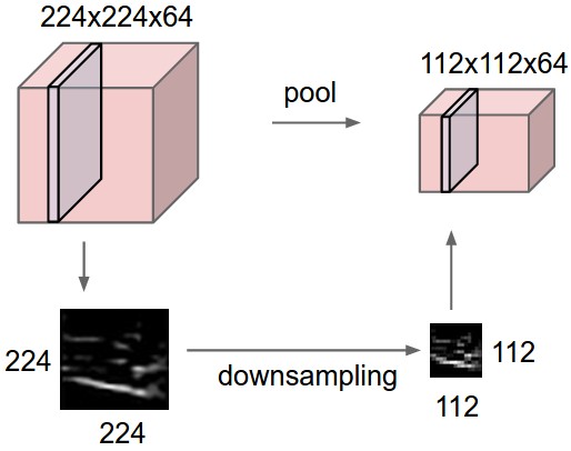
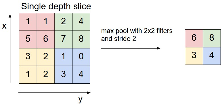Pooling layer downsamples the volume spatially, independently in each depth slice of the input volume. Left: In this example, the input volume of size [224x224x64] is pooled with filter size 2, stride 2 into output volume of size [112x112x64]. Notice that the volume depth is preserved. Right: The most common downsampling operation is max, giving rise to max pooling, here shown with a stride of 2. That is, each max is taken over 4 numbers (little 2x2 square).

Pooling 층은 입력 부피의 깊이 슬라이스마다 독립적으로 부피의 공간 크기를 줄인다. 왼쪽: 이 예에서는 [224x224x64] 크기의 입력 부피를 필터 크기 2, stride 2로 pooling해 [112x112x64] 크기의 출력 부피로 만든다. 부피의 깊이가 그대로 유지된다는 점에 유의하자. 오른쪽: 가장 흔한 다운샘플링 연산은 최댓값을 고르는 것이고 여기서 max pooling이 나왔다. 그림에서는 stride 2로 그렸다. 곧 최댓값 하나하나를 네 개의 수(작은 2x2 정사각형)에서 고른다.

Backpropagation. Recall from the backpropagation chapter that the backward pass for a max(x, y) operation has a simple interpretation as only routing the gradient to the input that had the highest value in the forward pass. Hence, during the forward pass of a pooling layer it is common to keep track of the index of the max activation (sometimes also called the switches) so that gradient routing is efficient during backpropagation.

역전파. 역전파 장에서 봤듯이 max(x, y) 연산의 역방향 진행은 간단하게 해석된다. 순전파에서 가장 큰 값이었던 입력 쪽으로만 기울기를 흘려보내면 된다. 그래서 pooling 층의 순전파 동안 최대 활성값의 인덱스(스위치라고 부르기도 한다)를 기록해두어, 역전파 때 기울기를 효율적으로 흘려보내는 것이 흔하다.

Getting rid of pooling. Many people dislike the pooling operation and think that we can get away without it. For example, Striving for Simplicity: The All Convolutional Net proposes to discard the pooling layer in favor of architecture that only consists of repeated CONV layers. To reduce the size of the representation they suggest using larger stride in CONV layer once in a while. Discarding pooling layers has also been found to be important in training good generative models, such as variational autoencoders (VAEs) or generative adversarial networks (GANs). It seems likely that future architectures will feature very few to no pooling layers.

pooling 없애기. pooling 연산을 싫어해서 그것 없이도 해낼 수 있다고 생각하는 사람이 많다. 예컨대 Striving for Simplicity: The All Convolutional Net은 pooling 층을 버리고 CONV 층만 반복해 쌓은 구조를 쓰자고 제안한다. 표현의 크기를 줄이기 위해서는 가끔 CONV 층에서 stride를 크게 쓰라고 권한다. pooling 층을 버리는 것은 변분 오토인코더(VAE)나 생성적 적대 신경망(GAN) 같은 좋은 생성 모델을 학습시킬 때도 중요하다는 사실이 밝혀졌다. 앞으로의 구조에는 pooling 층이 아주 적거나 아예 없을 가능성이 높아 보인다.

Normalization Layer

Many types of normalization layers have been proposed for use in ConvNet architectures, sometimes with the intentions of implementing inhibition schemes observed in the biological brain. However, these layers have since fallen out of favor because in practice their contribution has been shown to be minimal, if any. For various types of normalizations, see the discussion in Alex Krizhevsky’s cuda-convnet library API.

ConvNet 구조에 쓸 정규화(normalization) 층은 여러 종류가 제안되었고, 더러는 생물학적 뇌에서 관찰되는 억제 기전을 구현하려는 의도였다. 하지만 이 층들은 실제로 기여하는 바가 있다 해도 미미하다는 것이 드러나면서 이후 인기를 잃었다. 여러 종류의 정규화에 대해서는 Alex Krizhevsky의 cuda-convnet 라이브러리 API 설명을 보라.

Fully-connected layer

Neurons in a fully connected layer have full connections to all activations in the previous layer, as seen in regular Neural Networks. Their activations can hence be computed with a matrix multiplication followed by a bias offset. See the Neural Network section of the notes for more information.

완전 연결 층의 뉴런은 보통의 신경망에서 봤듯이 앞 층의 모든 활성값에 빠짐없이 연결된다. 따라서 이 뉴런들의 활성값은 행렬 곱을 하고 편향을 더하는 것으로 계산할 수 있다. 더 자세한 내용은 강의 노트의 신경망 절을 참고하자.

Converting FC layers to CONV layers

It is worth noting that the only difference between FC and CONV layers is that the neurons in the CONV layer are connected only to a local region in the input, and that many of the neurons in a CONV volume share parameters. However, the neurons in both layers still compute dot products, so their functional form is identical. Therefore, it turns out that it’s possible to convert between FC and CONV layers:

FC 층과 CONV 층의 유일한 차이는 CONV 층의 뉴런이 입력의 국소 영역에만 연결된다는 것, 그리고 CONV 부피의 많은 뉴런이 매개변수를 공유한다는 것뿐이라는 점을 짚어둘 만하다. 두 층의 뉴런 모두 여전히 내적을 계산하므로 함수의 형태는 똑같다. 따라서 FC 층과 CONV 층 사이를 서로 바꿀 수 있다는 결론이 나온다.

• For any CONV layer there is an FC layer that implements the same forward function. The weight matrix would be a large matrix that is mostly zero except for at certain blocks (due to local connectivity) where the weights in many of the blocks are equal (due to parameter sharing).
• Conversely, any FC layer can be converted to a CONV layer. For example, an FC layer with \(K = 4096\) that is looking at some input volume of size \(7 \times 7 \times 512\) can be equivalently expressed as a CONV layer with \(F = 7, P = 0, S = 1, K = 4096\). In other words, we are setting the filter size to be exactly the size of the input volume, and hence the output will simply be \(1 \times 1 \times 4096\) since only a single depth column “fits” across the input volume, giving identical result as the initial FC layer.

• 어떤 CONV 층이든 같은 순전파 함수를 구현하는 FC 층이 존재한다. 그 가중치 행렬은 대부분이 0인 커다란 행렬이 되는데, (국소 연결 때문에) 특정 블록에서만 0이 아니고 (매개변수 공유 때문에) 그 블록들 가운데 많은 수의 가중치가 서로 같다.
• 거꾸로 어떤 FC 층이든 CONV 층으로 바꿀 수 있다. 예컨대 크기 \(7 \times 7 \times 512\)인 입력 부피를 들여다보는 \(K = 4096\)짜리 FC 층은 \(F = 7, P = 0, S = 1, K = 4096\)인 CONV 층으로 똑같이 나타낼 수 있다. 다시 말해 필터 크기를 입력 부피의 크기와 정확히 같게 잡는 것이고, 그러면 입력 부피에 깊이 기둥이 딱 하나만 “들어맞으므로” 출력은 그냥 \(1 \times 1 \times 4096\)이 되어 원래 FC 층과 똑같은 결과를 낸다.

FC->CONV conversion. Of these two conversions, the ability to convert an FC layer to a CONV layer is particularly useful in practice. Consider a ConvNet architecture that takes a 224x224x3 image, and then uses a series of CONV layers and POOL layers to reduce the image to an activations volume of size 7x7x512 (in an AlexNet architecture that we’ll see later, this is done by use of 5 pooling layers that downsample the input spatially by a factor of two each time, making the final spatial size 224/2/2/2/2/2 = 7). From there, an AlexNet uses two FC layers of size 4096 and finally the last FC layers with 1000 neurons that compute the class scores. We can convert each of these three FC layers to CONV layers as described above:

FC를 CONV로 바꾸기. 이 두 변환 가운데 실제로 특히 쓸모 있는 것은 FC 층을 CONV 층으로 바꾸는 쪽이다. 224x224x3 이미지를 받아 CONV 층과 POOL 층을 죽 거치며 이미지를 7x7x512 크기의 활성값 부피로 줄이는 ConvNet 구조를 생각해보자(뒤에서 볼 AlexNet 구조에서는 입력의 공간 크기를 매번 절반으로 줄이는 pooling 층 5개로 이 일을 하며, 그래서 최종 공간 크기가 224/2/2/2/2/2 = 7이 된다). 거기서부터 AlexNet은 크기 4096짜리 FC 층 두 개를 쓰고, 마지막에 클래스 점수를 계산하는 뉴런 1000개짜리 FC 층을 둔다. 이 세 FC 층을 위에서 설명한 대로 각각 CONV 층으로 바꿀 수 있다.

• Replace the first FC layer that looks at [7x7x512] volume with a CONV layer that uses filter size \(F = 7\), giving output volume [1x1x4096].
• Replace the second FC layer with a CONV layer that uses filter size \(F = 1\), giving output volume [1x1x4096]
• Replace the last FC layer similarly, with \(F=1\), giving final output [1x1x1000]

• [7x7x512] 부피를 들여다보는 첫 FC 층을 필터 크기 \(F = 7\)인 CONV 층으로 바꾼다. 출력 부피는 [1x1x4096]이 된다.
• 두 번째 FC 층을 필터 크기 \(F = 1\)인 CONV 층으로 바꾼다. 출력 부피는 [1x1x4096]이다
• 마지막 FC 층도 마찬가지로 \(F=1\)로 바꾼다. 최종 출력은 [1x1x1000]이다

Each of these conversions could in practice involve manipulating (e.g. reshaping) the weight matrix \(W\) in each FC layer into CONV layer filters. It turns out that this conversion allows us to “slide” the original ConvNet very efficiently across many spatial positions in a larger image, in a single forward pass.

실제로 이런 변환을 하려면 각 FC 층의 가중치 행렬 \(W\)를 CONV 층 필터로 주무르는(예컨대 모양을 바꾸는) 작업이 필요할 수 있다. 그런데 이 변환 덕분에 원래의 ConvNet을 더 큰 이미지의 여러 공간 위치에 걸쳐 아주 효율적으로, 그것도 순전파 한 번에 “미끄러뜨릴” 수 있게 된다.

For example, if 224x224 image gives a volume of size [7x7x512] - i.e. a reduction by 32, then forwarding an image of size 384x384 through the converted architecture would give the equivalent volume in size [12x12x512], since 384/32 = 12. Following through with the next 3 CONV layers that we just converted from FC layers would now give the final volume of size [6x6x1000], since (12 - 7)/1 + 1 = 6. Note that instead of a single vector of class scores of size [1x1x1000], we’re now getting an entire 6x6 array of class scores across the 384x384 image.

예컨대 224x224 이미지가 [7x7x512] 크기의 부피를 낸다면, 곧 크기가 32배로 줄어든다면, 384x384 크기의 이미지를 바꾼 구조에 넣었을 때 그에 대응하는 부피는 384/32 = 12이므로 [12x12x512]가 된다. 방금 FC 층에서 바꿔놓은 세 CONV 층까지 이어서 통과시키면 (12 - 7)/1 + 1 = 6이므로 최종 부피는 [6x6x1000] 크기가 된다. 크기 [1x1x1000]인 클래스 점수 벡터 하나 대신, 이제 384x384 이미지 전체에 걸친 6x6짜리 클래스 점수 배열을 통째로 얻는다는 점에 유의하자.

Evaluating the original ConvNet (with FC layers) independently across 224x224 crops of the 384x384 image in strides of 32 pixels gives an identical result to forwarding the converted ConvNet one time.

384x384 이미지에서 32픽셀 stride로 잘라낸 224x224 조각들에 원래의 (FC 층을 가진) ConvNet을 따로따로 적용한 결과는, 바꾼 ConvNet을 한 번 통과시킨 결과와 똑같다.

Naturally, forwarding the converted ConvNet a single time is much more efficient than iterating the original ConvNet over all those 36 locations, since the 36 evaluations share computation. This trick is often used in practice to get better performance, where for example, it is common to resize an image to make it bigger, use a converted ConvNet to evaluate the class scores at many spatial positions and then average the class scores.

당연히 바꾼 ConvNet을 한 번 통과시키는 쪽이 원래의 ConvNet을 그 36개 위치마다 되풀이해 돌리는 것보다 훨씬 효율적이다. 36번의 평가가 계산을 공유하기 때문이다. 이 요령은 성능을 더 끌어올리려고 실제로 자주 쓰인다. 예컨대 이미지를 더 크게 키운 다음 바꾼 ConvNet으로 여러 공간 위치에서 클래스 점수를 구하고 그 점수들을 평균 내는 식이다.

역주. 36이라는 수는 앞 문단의 [6x6x1000]에서 나온다. 6x6짜리 점수 배열의 칸 하나하나가 원래 이미지에서 224x224 조각 하나를 본 결과이고, 이웃한 칸 사이의 간격은 이 ConvNet이 공간 크기를 줄인 배수인 32픽셀이다. 실제로 맞아떨어지는지 세어보면, 여섯 번째 조각의 왼쪽 끝이 5*32 = 160이고 거기에 조각의 폭 224를 더하면 384로 이미지의 오른쪽 끝에 정확히 닿는다. 가로 6칸에 세로 6칸이니 조각은 모두 36개이며, 바꾸지 않은 ConvNet으로 같은 결과를 얻으려면 순전파를 36번 해야 한다는 뜻이다.

Lastly, what if we wanted to efficiently apply the original ConvNet over the image but at a stride smaller than 32 pixels? We could achieve this with multiple forward passes. For example, note that if we wanted to use a stride of 16 pixels we could do so by combining the volumes received by forwarding the converted ConvNet twice: First over the original image and second over the image but with the image shifted spatially by 16 pixels along both width and height.

마지막으로, 원래의 ConvNet을 이미지 위에 효율적으로 적용하되 stride를 32픽셀보다 작게 하고 싶다면 어떻게 할까? 순전파를 여러 번 하면 된다. 예컨대 stride를 16픽셀로 하고 싶다면, 바꾼 ConvNet을 두 번 통과시켜 얻은 부피를 합치면 된다. 한 번은 원래 이미지에, 다른 한 번은 가로세로 양쪽으로 16픽셀씩 공간적으로 옮긴 이미지에 적용하는 것이다.

• An IPython Notebook on Net Surgery shows how to perform the conversion in practice, in code (using Caffe)

• Net Surgery IPython Notebook은 이 변환을 실제 코드에서 (Caffe로) 어떻게 하는지 보여준다

ConvNet Architectures

We have seen that Convolutional Networks are commonly made up of only three layer types: CONV, POOL (we assume Max pool unless stated otherwise) and FC (short for fully-connected). We will also explicitly write the RELU activation function as a layer, which applies elementwise non-linearity. In this section we discuss how these are commonly stacked together to form entire ConvNets.

합성곱 신경망이 흔히 CONV, POOL(따로 말이 없으면 Max pooling으로 본다), FC(완전 연결의 줄임말)라는 세 가지 층으로만 이루어진다는 것을 봤다. 여기에 더해 원소별로 비선형성을 적용하는 RELU 활성화 함수도 하나의 층으로 명시해 쓰겠다. 이 절에서는 이것들을 흔히 어떻게 쌓아 ConvNet 전체를 만드는지 이야기한다.

Layer Patterns

The most common form of a ConvNet architecture stacks a few CONV-RELU layers, follows them with POOL layers, and repeats this pattern until the image has been merged spatially to a small size. At some point, it is common to transition to fully-connected layers. The last fully-connected layer holds the output, such as the class scores. In other words, the most common ConvNet architecture follows the pattern:

ConvNet 구조에서 가장 흔한 형태는 CONV-RELU 층을 몇 개 쌓고 그 뒤에 POOL 층을 붙이는 것을, 이미지가 공간적으로 충분히 작아질 때까지 되풀이하는 것이다. 어느 지점에 이르면 완전 연결 층으로 넘어가는 것이 보통이다. 마지막 완전 연결 층이 클래스 점수 같은 출력을 담는다. 다시 말해 가장 흔한 ConvNet 구조는 다음 패턴을 따른다.

INPUT -> [[CONV -> RELU]*N -> POOL?]*M -> [FC -> RELU]*K -> FC

INPUT -> [[CONV -> RELU]*N -> POOL?]*M -> [FC -> RELU]*K -> FC

where the * indicates repetition, and the POOL? indicates an optional pooling layer. Moreover, N >= 0 (and usually N <= 3), M >= 0, K >= 0 (and usually K < 3). For example, here are some common ConvNet architectures you may see that follow this pattern:

여기서 *는 반복을 뜻하고 POOL?은 pooling 층이 있을 수도 없을 수도 있다는 뜻이다. 또한 N >= 0(보통은 N <= 3), M >= 0, K >= 0(보통은 K < 3)이다. 예컨대 이 패턴을 따르는 흔한 ConvNet 구조로 다음과 같은 것들을 볼 수 있다.

• INPUT -> FC, implements a linear classifier. Here N = M = K = 0.
• INPUT -> CONV -> RELU -> FC
• INPUT -> [CONV -> RELU -> POOL]*2 -> FC -> RELU -> FC. Here we see that there is a single CONV layer between every POOL layer.
• INPUT -> [CONV -> RELU -> CONV -> RELU -> POOL]*3 -> [FC -> RELU]*2 -> FC Here we see two CONV layers stacked before every POOL layer. This is generally a good idea for larger and deeper networks, because multiple stacked CONV layers can develop more complex features of the input volume before the destructive pooling operation.

• INPUT -> FC는 선형 분류기를 구현한다. 여기서는 N = M = K = 0이다.
• INPUT -> CONV -> RELU -> FC
• INPUT -> [CONV -> RELU -> POOL]*2 -> FC -> RELU -> FC. 여기서는 POOL 층 사이마다 CONV 층이 하나씩 있다.
• INPUT -> [CONV -> RELU -> CONV -> RELU -> POOL]*3 -> [FC -> RELU]*2 -> FC 여기서는 POOL 층 앞마다 CONV 층이 두 개씩 쌓여 있다. 더 크고 깊은 신경망에서는 대체로 이렇게 하는 것이 좋다. CONV 층을 여러 개 쌓으면 정보를 깎아내는 pooling 연산을 만나기 전에 입력 부피에서 더 복잡한 특징을 뽑아낼 수 있기 때문이다.

Prefer a stack of small filter CONV to one large receptive field CONV layer. Suppose that you stack three 3x3 CONV layers on top of each other (with non-linearities in between, of course). In this arrangement, each neuron on the first CONV layer has a 3x3 view of the input volume. A neuron on the second CONV layer has a 3x3 view of the first CONV layer, and hence by extension a 5x5 view of the input volume. Similarly, a neuron on the third CONV layer has a 3x3 view of the 2nd CONV layer, and hence a 7x7 view of the input volume. Suppose that instead of these three layers of 3x3 CONV, we only wanted to use a single CONV layer with 7x7 receptive fields. These neurons would have a receptive field size of the input volume that is identical in spatial extent (7x7), but with several disadvantages. First, the neurons would be computing a linear function over the input, while the three stacks of CONV layers contain non-linearities that make their features more expressive. Second, if we suppose that all the volumes have \(C\) channels, then it can be seen that the single 7x7 CONV layer would contain \(C \times (7 \times 7 \times C) = 49 C^2\) parameters, while the three 3x3 CONV layers would only contain \(3 \times (C \times (3 \times 3 \times C)) = 27 C^2\) parameters. Intuitively, stacking CONV layers with tiny filters as opposed to having one CONV layer with big filters allows us to express more powerful features of the input, and with fewer parameters. As a practical disadvantage, we might need more memory to hold all the intermediate CONV layer results if we plan to do backpropagation.

수용 영역이 큰 CONV 층 하나보다 작은 필터 CONV 층을 쌓는 쪽이 낫다. 3x3 CONV 층 세 개를 위아래로 쌓았다고 하자(물론 사이사이에 비선형성이 들어간다). 이 배치에서 첫 CONV 층의 각 뉴런은 입력 부피를 3x3만큼 본다. 두 번째 CONV 층의 뉴런은 첫 CONV 층을 3x3만큼 보므로, 그것을 거슬러 올라가면 입력 부피를 5x5만큼 보는 셈이다. 마찬가지로 세 번째 CONV 층의 뉴런은 두 번째 CONV 층을 3x3만큼 보므로 입력 부피는 7x7만큼 본다. 이 3x3 CONV 층 세 개 대신 7x7 수용 영역을 가진 CONV 층 하나만 쓰고 싶다고 해보자. 이 뉴런들이 입력 부피에서 보는 수용 영역의 공간적 크기는 (7x7로) 똑같겠지만 불리한 점이 몇 가지 있다. 첫째, 이 뉴런들은 입력에 대해 선형 함수를 계산하는 반면, 세 겹으로 쌓은 CONV 층에는 비선형성이 들어 있어 특징이 더 풍부하게 표현된다. 둘째, 모든 부피의 채널 수가 \(C\)라고 하면, 7x7 CONV 층 하나는 \(C \times (7 \times 7 \times C) = 49 C^2\)개의 매개변수를 갖는 반면 3x3 CONV 층 세 개는 \(3 \times (C \times (3 \times 3 \times C)) = 27 C^2\)개만 갖는다는 것을 알 수 있다. 직관적으로 보면, 큰 필터의 CONV 층 하나를 두는 대신 작은 필터의 CONV 층을 쌓으면 입력의 더 강력한 특징을 더 적은 매개변수로 표현할 수 있다. 실용적인 단점을 들자면, 역전파를 할 계획이라면 중간 CONV 층의 결과를 모두 들고 있어야 하므로 메모리가 더 필요할 수 있다.

Recent departures. It should be noted that the conventional paradigm of a linear list of layers has recently been challenged, in Google’s Inception architectures and also in current (state of the art) Residual Networks from Microsoft Research Asia. Both of these (see details below in case studies section) feature more intricate and different connectivity structures.

최근의 이탈. 층을 일렬로 늘어놓는 기존의 틀은 최근 Google의 Inception 구조와 Microsoft Research Asia의 (현재 최고 성능인) Residual Network에서 도전받고 있다는 점을 짚어둘 만하다. 둘 다 (자세한 내용은 아래 사례 연구 절을 보라) 더 복잡하고 색다른 연결 구조를 갖고 있다.

In practice: use whatever works best on ImageNet. If you’re feeling a bit of a fatigue in thinking about the architectural decisions, you’ll be pleased to know that in 90% or more of applications you should not have to worry about these. I like to summarize this point as “don’t be a hero”: Instead of rolling your own architecture for a problem, you should look at whatever architecture currently works best on ImageNet, download a pretrained model and finetune it on your data. You should rarely ever have to train a ConvNet from scratch or design one from scratch. I also made this point at the Deep Learning school.

실전에서는 ImageNet에서 가장 잘 되는 것을 쓴다. 구조를 어떻게 정할지 고민하는 데 슬슬 지쳤다면, 응용의 90% 이상에서는 이런 걱정을 할 필요가 없다는 사실이 반가울 것이다. 나는 이 점을 “영웅이 되려 하지 말라”로 요약하곤 한다. 문제마다 자기만의 구조를 지어내는 대신, 지금 ImageNet에서 가장 잘 되는 구조를 찾아 미리 학습된 모델을 내려받아 자기 데이터에 fine-tuning하면 된다. ConvNet을 맨바닥에서 학습시키거나 맨바닥에서 설계할 일은 거의 없어야 한다. Deep Learning school에서도 이 이야기를 했다.

Layer Sizing Patterns

Until now we’ve omitted mentions of common hyperparameters used in each of the layers in a ConvNet. We will first state the common rules of thumb for sizing the architectures and then follow the rules with a discussion of the notation:

지금까지는 ConvNet의 각 층에서 흔히 쓰는 하이퍼파라미터 이야기를 빼놓았다. 먼저 구조의 크기를 잡는 흔한 어림법을 늘어놓고, 그다음에 그 규칙들을 두고 표기 이야기를 이어가겠다.

The input layer (that contains the image) should be divisible by 2 many times. Common numbers include 32 (e.g. CIFAR-10), 64, 96 (e.g. STL-10), or 224 (e.g. common ImageNet ConvNets), 384, and 512.

(이미지를 담는) 입력층은 2로 여러 번 나누어떨어져야 한다. 흔한 수로는 32(예컨대 CIFAR-10), 64, 96(예컨대 STL-10), 224(예컨대 흔한 ImageNet ConvNet), 384, 512가 있다.

The conv layers should be using small filters (e.g. 3x3 or at most 5x5), using a stride of \(S = 1\), and crucially, padding the input volume with zeros in such way that the conv layer does not alter the spatial dimensions of the input. That is, when \(F = 3\), then using \(P = 1\) will retain the original size of the input. When \(F = 5\), \(P = 2\). For a general \(F\), it can be seen that \(P = (F - 1) / 2\) preserves the input size. If you must use bigger filter sizes (such as 7x7 or so), it is only common to see this on the very first conv layer that is looking at the input image.

conv 층은 작은 필터(예컨대 3x3, 커도 5x5)를 쓰고 stride는 \(S = 1\)로 하며, 결정적으로 conv 층이 입력의 공간 차원을 바꾸지 않도록 입력 부피에 0을 덧대야 한다. 곧 \(F = 3\)일 때 \(P = 1\)을 쓰면 입력의 원래 크기가 유지된다. \(F = 5\)이면 \(P = 2\)다. 일반적인 \(F\)에 대해서는 \(P = (F - 1) / 2\)가 입력 크기를 보존한다는 것을 알 수 있다. 더 큰 필터 크기(7x7쯤)를 꼭 써야 한다면, 그런 경우는 입력 이미지를 직접 들여다보는 맨 첫 conv 층에서만 보는 것이 보통이다.

The pool layers are in charge of downsampling the spatial dimensions of the input. The most common setting is to use max-pooling with 2x2 receptive fields (i.e. \(F = 2\)), and with a stride of 2 (i.e. \(S = 2\)). Note that this discards exactly 75% of the activations in an input volume (due to downsampling by 2 in both width and height). Another slightly less common setting is to use 3x3 receptive fields with a stride of 2, but this makes “fitting” more complicated (e.g., a 32x32x3 layer would require zero padding to be used with a max-pooling layer with 3x3 receptive field and stride 2). It is very uncommon to see receptive field sizes for max pooling that are larger than 3 because the pooling is then too lossy and aggressive. This usually leads to worse performance.

pool 층은 입력의 공간 차원을 다운샘플링하는 역할을 맡는다. 가장 흔한 설정은 2x2 수용 영역(곧 \(F = 2\))에 stride 2(곧 \(S = 2\))로 max-pooling을 쓰는 것이다. 이렇게 하면 (가로세로 양쪽으로 2배씩 다운샘플링하므로) 입력 부피 활성값의 정확히 75%를 버리게 된다는 점에 유의하자. 조금 덜 흔한 또 다른 설정은 3x3 수용 영역에 stride 2를 쓰는 것인데, 이러면 크기를 “맞추는” 일이 더 까다로워진다(예컨대 32x32x3 층에 3x3 수용 영역과 stride 2인 max-pooling 층을 쓰려면 zero padding이 필요하다). max pooling의 수용 영역 크기가 3보다 큰 경우는 아주 드문데, 그렇게 하면 pooling이 정보를 너무 많이 잃고 지나치게 공격적이기 때문이다. 그러면 대개 성능이 나빠진다.

Reducing sizing headaches. The scheme presented above is pleasing because all the CONV layers preserve the spatial size of their input, while the POOL layers alone are in charge of down-sampling the volumes spatially. In an alternative scheme where we use strides greater than 1 or don’t zero-pad the input in CONV layers, we would have to very carefully keep track of the input volumes throughout the CNN architecture and make sure that all strides and filters “work out”, and that the ConvNet architecture is nicely and symmetrically wired.

크기 때문에 머리 아플 일 줄이기. 위에 제시한 방식이 마음에 드는 이유는 CONV 층이 모두 입력의 공간 크기를 보존하고, 부피의 공간 크기를 줄이는 일은 POOL 층이 도맡기 때문이다. 그 대신 CONV 층에서 stride를 1보다 크게 쓰거나 입력에 0을 덧대지 않는 방식을 택하면, CNN 구조 전체에 걸쳐 입력 부피를 아주 조심스럽게 따라가며 모든 stride와 필터가 “맞아떨어지는지”, 그리고 ConvNet 구조가 깔끔하고 대칭적으로 이어지는지 확인해야 한다.

Why use stride of 1 in CONV? Smaller strides work better in practice. Additionally, as already mentioned stride 1 allows us to leave all spatial down-sampling to the POOL layers, with the CONV layers only transforming the input volume depth-wise.

CONV에서 왜 stride를 1로 쓰는가? 작은 stride가 실제로 더 잘 동작한다. 게다가 이미 말했듯이 stride를 1로 두면 공간 방향의 다운샘플링을 전부 POOL 층에 맡기고 CONV 층은 입력 부피를 깊이 방향으로만 변환하게 할 수 있다.

Why use padding? In addition to the aforementioned benefit of keeping the spatial sizes constant after CONV, doing this actually improves performance. If the CONV layers were to not zero-pad the inputs and only perform valid convolutions, then the size of the volumes would reduce by a small amount after each CONV, and the information at the borders would be “washed away” too quickly.

왜 padding을 쓰는가? 앞서 말한 것처럼 CONV 이후에도 공간 크기를 그대로 유지할 수 있다는 이점에 더해, 이렇게 하면 실제로 성능도 좋아진다. CONV 층이 입력에 0을 덧대지 않고 유효 합성곱만 수행한다면 CONV를 지날 때마다 부피의 크기가 조금씩 줄어들고, 테두리의 정보가 너무 빠르게 “씻겨 나가버린다”.

Compromising based on memory constraints. In some cases (especially early in the ConvNet architectures), the amount of memory can build up very quickly with the rules of thumb presented above. For example, filtering a 224x224x3 image with three 3x3 CONV layers with 64 filters each and padding 1 would create three activation volumes of size [224x224x64]. This amounts to a total of about 10 million activations, or 72MB of memory (per image, for both activations and gradients). Since GPUs are often bottlenecked by memory, it may be necessary to compromise. In practice, people prefer to make the compromise at only the first CONV layer of the network. For example, one compromise might be to use a first CONV layer with filter sizes of 7x7 and stride of 2 (as seen in a ZF net). As another example, an AlexNet uses filter sizes of 11x11 and stride of 4.

메모리 제약에 맞춰 타협하기. 어떤 경우에는(특히 ConvNet 구조의 앞쪽에서는) 위에 제시한 어림법을 따르면 메모리 사용량이 아주 빠르게 불어난다. 예컨대 224x224x3 이미지를 필터 64개짜리 3x3 CONV 층 세 개로 패딩 1을 주어 거르면 [224x224x64] 크기의 활성값 부피가 세 개 생긴다. 이는 활성값을 모두 합쳐 약 1000만 개, 메모리로는 72MB(이미지 한 장당, 활성값과 기울기를 합쳐)에 해당한다. GPU는 메모리에서 병목이 걸리는 일이 많으므로 타협이 필요할 수 있다. 실제로는 신경망의 첫 CONV 층에서만 타협하는 쪽을 선호한다. 예컨대 (ZF net에서 보듯이) 첫 CONV 층의 필터 크기를 7x7로, stride를 2로 잡는 식의 타협이 있다. 또 다른 예로 AlexNet은 필터 크기 11x11에 stride 4를 쓴다.

역주. 72MB가 어디서 나오는지 한 번 세어두면 이 타협의 무게가 실감된다. [224x224x64] 부피 하나에 224*224*64 = 3,211,264개의 활성값이 있고 그런 부피가 셋이니 9,633,792개, 원문이 말한 “약 1000만 개”다. 부동소수점 하나가 4바이트이므로 활성값만 약 36.8MiB이고, 역전파를 하려면 같은 크기의 기울기를 함께 들고 있어야 하므로 두 배인 약 73.5MiB가 된다. 원문의 72MB는 이 값을 어림한 것이다.

중요한 것은 이것이 이미지 한 장, 그것도 신경망의 앞쪽 세 층만 센 값이라는 점이다. 배치 크기를 32로 잡으면 이 세 층만으로 2.3GB를 쓴다. 첫 CONV 층에서 stride를 2로 올리는 타협이 그 자리에서 왜 그렇게 값어치를 하는지가 여기서 보인다. 첫 층의 공간 크기가 절반으로 줄면 그 부피의 활성값은 4분의 1이 된다.

Case studies

There are several architectures in the field of Convolutional Networks that have a name. The most common are:

합성곱 신경망 분야에는 이름이 붙은 구조가 여럿 있다. 가장 흔한 것들은 다음과 같다.

• LeNet. The first successful applications of Convolutional Networks were developed by Yann LeCun in 1990’s. Of these, the best known is the LeNet architecture that was used to read zip codes, digits, etc.
• AlexNet. The first work that popularized Convolutional Networks in Computer Vision was the AlexNet, developed by Alex Krizhevsky, Ilya Sutskever and Geoff Hinton. The AlexNet was submitted to the ImageNet ILSVRC challenge in 2012 and significantly outperformed the second runner-up (top 5 error of 16% compared to runner-up with 26% error). The Network had a very similar architecture to LeNet, but was deeper, bigger, and featured Convolutional Layers stacked on top of each other (previously it was common to only have a single CONV layer always immediately followed by a POOL layer).
• ZF Net. The ILSVRC 2013 winner was a Convolutional Network from Matthew Zeiler and Rob Fergus. It became known as the ZFNet (short for Zeiler & Fergus Net). It was an improvement on AlexNet by tweaking the architecture hyperparameters, in particular by expanding the size of the middle convolutional layers and making the stride and filter size on the first layer smaller.
• GoogLeNet. The ILSVRC 2014 winner was a Convolutional Network from Szegedy et al. from Google. Its main contribution was the development of an Inception Module that dramatically reduced the number of parameters in the network (4M, compared to AlexNet with 60M). Additionally, this paper uses Average Pooling instead of Fully Connected layers at the top of the ConvNet, eliminating a large amount of parameters that do not seem to matter much. There are also several followup versions to the GoogLeNet, most recently Inception-v4.
• VGGNet. The runner-up in ILSVRC 2014 was the network from Karen Simonyan and Andrew Zisserman that became known as the VGGNet. Its main contribution was in showing that the depth of the network is a critical component for good performance. Their final best network contains 16 CONV/FC layers and, appealingly, features an extremely homogeneous architecture that only performs 3x3 convolutions and 2x2 pooling from the beginning to the end. Their pretrained model is available for plug and play use in Caffe. A downside of the VGGNet is that it is more expensive to evaluate and uses a lot more memory and parameters (140M). Most of these parameters are in the first fully connected layer, and it was since found that these FC layers can be removed with no performance downgrade, significantly reducing the number of necessary parameters.
• ResNet. Residual Network developed by Kaiming He et al. was the winner of ILSVRC 2015. It features special skip connections and a heavy use of batch normalization. The architecture is also missing fully connected layers at the end of the network. The reader is also referred to Kaiming’s presentation (video, slides), and some recent experiments that reproduce these networks in Torch. ResNets are currently by far state of the art Convolutional Neural Network models and are the default choice for using ConvNets in practice (as of May 10, 2016). In particular, also see more recent developments that tweak the original architecture from Kaiming He et al. Identity Mappings in Deep Residual Networks (published March 2016).

• LeNet. 합성곱 신경망이 처음으로 성공을 거둔 응용은 1990년대에 Yann LeCun이 개발한 것들이다. 그중 가장 잘 알려진 것이 우편번호나 숫자 따위를 읽는 데 쓰인 LeNet 구조다.
• AlexNet. 컴퓨터 비전에서 합성곱 신경망을 널리 알린 첫 연구는 Alex Krizhevsky, Ilya Sutskever, Geoff Hinton이 개발한 AlexNet이다. AlexNet은 2012년 ImageNet ILSVRC 챌린지에 출품되어 2위를 큰 차이로 앞질렀다(상위 5개 오류율이 16%로, 26%였던 2위보다 훨씬 낮았다). 이 신경망은 LeNet과 아주 비슷한 구조였지만 더 깊고 더 컸으며, 합성곱 층을 여러 개 위아래로 쌓은 것이 특징이었다(그전에는 CONV 층 하나 뒤에 곧바로 POOL 층이 붙는 형태만 흔했다).
• ZF Net. ILSVRC 2013 우승은 Matthew Zeiler와 Rob Fergus의 합성곱 신경망이었다. 이것은 ZFNet(Zeiler & Fergus Net의 줄임말)으로 알려졌다. AlexNet의 구조 하이퍼파라미터를 손봐 개선한 것으로, 특히 가운데 합성곱 층들의 크기를 키우고 첫 층의 stride와 필터 크기를 줄였다.
• GoogLeNet. ILSVRC 2014 우승은 Google의 Szegedy et al.이 만든 합성곱 신경망이었다. 가장 큰 기여는 신경망의 매개변수 개수를 극적으로 줄인 Inception 모듈을 만들어낸 것이다(AlexNet의 6000만 개에 비해 400만 개다). 또한 이 논문은 ConvNet 꼭대기에서 완전 연결 층 대신 Average Pooling을 써서, 별로 중요하지 않아 보이는 매개변수를 대량으로 걷어냈다. GoogLeNet에는 후속 버전도 여럿 있으며 가장 최근 것은 Inception-v4다.
• VGGNet. ILSVRC 2014 준우승은 Karen Simonyan과 Andrew Zisserman의 신경망으로 VGGNet으로 알려졌다. 가장 큰 기여는 좋은 성능에 신경망의 깊이가 결정적인 요소임을 보인 것이다. 이들의 최종 최고 신경망은 CONV/FC 층 16개로 이루어져 있고, 처음부터 끝까지 3x3 합성곱과 2x2 pooling만 하는 대단히 균질한 구조라는 점이 마음에 든다. 이들의 미리 학습된 모델은 Caffe에서 바로 가져다 쓸 수 있다. VGGNet의 단점은 평가 비용이 더 크고 메모리와 매개변수를 훨씬 많이 쓴다는 것이다(1억 4000만 개). 이 매개변수의 대부분은 첫 번째 완전 연결 층에 있는데, 이후 이 FC 층들을 성능 저하 없이 걷어낼 수 있다는 것이 밝혀져 필요한 매개변수 개수가 크게 줄었다.
• ResNet. Kaiming He et al.이 개발한 Residual Network는 ILSVRC 2015 우승작이다. 특별한 skip connection과 batch normalization의 적극적인 사용이 특징이다. 이 구조에는 신경망 끝의 완전 연결 층도 없다. Kaiming의 발표(영상, 슬라이드)와, 이 신경망들을 Torch로 재현한 최근 실험도 함께 보기를 권한다. ResNet은 (2016년 5월 10일 기준으로) 현재 압도적인 최고 성능의 합성곱 신경망 모델이며 실전에서 ConvNet을 쓸 때의 기본 선택지다. 특히 원래 구조를 손본 더 최근의 진전인 Kaiming He et al. Identity Mappings in Deep Residual Networks(2016년 3월 발표)도 함께 보라.

VGGNet in detail. Lets break down the VGGNet in more detail as a case study. The whole VGGNet is composed of CONV layers that perform 3x3 convolutions with stride 1 and pad 1, and of POOL layers that perform 2x2 max pooling with stride 2 (and no padding). We can write out the size of the representation at each step of the processing and keep track of both the representation size and the total number of weights:

VGGNet 자세히 보기. 사례 연구로 VGGNet을 좀 더 자세히 뜯어보자. VGGNet 전체는 stride 1, 패딩 1로 3x3 합성곱을 하는 CONV 층과, 패딩 없이 stride 2로 2x2 max pooling을 하는 POOL 층으로 이루어져 있다. 처리 과정의 단계마다 표현의 크기를 적어보면서 표현의 크기와 전체 가중치 개수를 함께 따라가볼 수 있다.

INPUT: [224x224x3]        memory:  224*224*3=150K   weights: 0
CONV3-64: [224x224x64]  memory:  224*224*64=3.2M   weights: (3*3*3)*64 = 1,728
CONV3-64: [224x224x64]  memory:  224*224*64=3.2M   weights: (3*3*64)*64 = 36,864
POOL2: [112x112x64]  memory:  112*112*64=800K   weights: 0
CONV3-128: [112x112x128]  memory:  112*112*128=1.6M   weights: (3*3*64)*128 = 73,728
CONV3-128: [112x112x128]  memory:  112*112*128=1.6M   weights: (3*3*128)*128 = 147,456
POOL2: [56x56x128]  memory:  56*56*128=400K   weights: 0
CONV3-256: [56x56x256]  memory:  56*56*256=800K   weights: (3*3*128)*256 = 294,912
CONV3-256: [56x56x256]  memory:  56*56*256=800K   weights: (3*3*256)*256 = 589,824
CONV3-256: [56x56x256]  memory:  56*56*256=800K   weights: (3*3*256)*256 = 589,824
POOL2: [28x28x256]  memory:  28*28*256=200K   weights: 0
CONV3-512: [28x28x512]  memory:  28*28*512=400K   weights: (3*3*256)*512 = 1,179,648
CONV3-512: [28x28x512]  memory:  28*28*512=400K   weights: (3*3*512)*512 = 2,359,296
CONV3-512: [28x28x512]  memory:  28*28*512=400K   weights: (3*3*512)*512 = 2,359,296
POOL2: [14x14x512]  memory:  14*14*512=100K   weights: 0
CONV3-512: [14x14x512]  memory:  14*14*512=100K   weights: (3*3*512)*512 = 2,359,296
CONV3-512: [14x14x512]  memory:  14*14*512=100K   weights: (3*3*512)*512 = 2,359,296
CONV3-512: [14x14x512]  memory:  14*14*512=100K   weights: (3*3*512)*512 = 2,359,296
POOL2: [7x7x512]  memory:  7*7*512=25K  weights: 0
FC: [1x1x4096]  memory:  4096  weights: 7*7*512*4096 = 102,760,448
FC: [1x1x4096]  memory:  4096  weights: 4096*4096 = 16,777,216
FC: [1x1x1000]  memory:  1000 weights: 4096*1000 = 4,096,000

TOTAL memory: 24M * 4 bytes ~= 93MB / image (only forward! ~*2 for bwd)
TOTAL params: 138M parameters

As is common with Convolutional Networks, notice that most of the memory (and also compute time) is used in the early CONV layers, and that most of the parameters are in the last FC layers. In this particular case, the first FC layer contains 100M weights, out of a total of 140M.

합성곱 신경망에서 흔히 그렇듯이 메모리(그리고 계산 시간)의 대부분이 앞쪽 CONV 층에서 쓰이고, 매개변수의 대부분은 마지막 FC 층에 있다는 점에 유의하자. 이 경우에는 전체 1억 4000만 개 가운데 1억 개의 가중치가 첫 FC 층에 들어 있다.

보충: VGGNet 표의 두 열을 직접 더해보기

원문 표는 층마다 메모리와 가중치를 적어놓고 맨 아래에 합계만 툭 던진다. 그 합계가 정말 표에서 나오는지, 그리고 바로 위 문단이 말하는 “전체 1억 4000만 개 가운데 1억 개”가 표의 어느 줄인지는 직접 더해봐야 보인다. 원문 표를 그대로 옮겨 두 열을 합산해봤다. 원문 코드는 한 글자도 고치지 않았고, 아래 코드는 Python 3으로 새로 썼다.

# 원문 표를 그대로 옮겼다: (층 이름, 활성값 부피의 모양, 가중치 개수)
layers = [
    ('INPUT',     (224, 224, 3),   0),
    ('CONV3-64',  (224, 224, 64),  (3*3*3)*64),
    ('CONV3-64',  (224, 224, 64),  (3*3*64)*64),
    ('POOL2',     (112, 112, 64),  0),
    ('CONV3-128', (112, 112, 128), (3*3*64)*128),
    ('CONV3-128', (112, 112, 128), (3*3*128)*128),
    ('POOL2',     (56, 56, 128),   0),
    ('CONV3-256', (56, 56, 256),   (3*3*128)*256),
    ('CONV3-256', (56, 56, 256),   (3*3*256)*256),
    ('CONV3-256', (56, 56, 256),   (3*3*256)*256),
    ('POOL2',     (28, 28, 256),   0),
    ('CONV3-512', (28, 28, 512),   (3*3*256)*512),
    ('CONV3-512', (28, 28, 512),   (3*3*512)*512),
    ('CONV3-512', (28, 28, 512),   (3*3*512)*512),
    ('POOL2',     (14, 14, 512),   0),
    ('CONV3-512', (14, 14, 512),   (3*3*512)*512),
    ('CONV3-512', (14, 14, 512),   (3*3*512)*512),
    ('CONV3-512', (14, 14, 512),   (3*3*512)*512),
    ('POOL2',     (7, 7, 512),     0),
    ('FC',        (1, 1, 4096),    7*7*512*4096),
    ('FC',        (1, 1, 4096),    4096*4096),
    ('FC',        (1, 1, 1000),    4096*1000),
]

acts = [w*h*d for _, (w, h, d), _ in layers]
wts = [n for _, _, n in layers]
MB = 1024 * 1024

print('활성값 합계 : {:,}개 ({:.1f}M) → 순전파만 {:.0f}MB'.format(
    sum(acts), sum(acts)/1e6, sum(acts)*4/MB))
print('원문 합계줄 : 24M → 순전파만 {:.0f}MB'.format(24e6*4/MB))
print('가중치 합계 : {:,}개 ({:.0f}M)'.format(sum(wts), sum(wts)/1e6))
print()
print('첫 CONV 두 층의 활성값이 전체에서 차지하는 비율 : {:.0%}'.format(
    (acts[1]+acts[2])/sum(acts)))
print('첫 FC 층의 가중치가 전체에서 차지하는 비율       : {:.0%}'.format(wts[19]/sum(wts)))
print('FC 층 셋의 가중치가 전체에서 차지하는 비율       : {:.0%}'.format(
    sum(wts[19:])/sum(wts)))

활성값 합계 : 15,237,608개 (15.2M) → 순전파만 58MB
원문 합계줄 : 24M → 순전파만 92MB
가중치 합계 : 138,344,128개 (138M)

첫 CONV 두 층의 활성값이 전체에서 차지하는 비율 : 42%
첫 FC 층의 가중치가 전체에서 차지하는 비율       : 74%
FC 층 셋의 가중치가 전체에서 차지하는 비율       : 89%

가중치 쪽은 표와 합계줄이 정확히 맞는다. 138,344,128개이고 원문의 TOTAL params: 138M과 같다. 첫 FC 층 하나가 그중 74%를 가져가고 FC 층 셋을 합치면 89%다. 원문 문단이 “1억 4000만 개 가운데 1억 개”라고 한 것은 이 74%를 어림한 말이며, 표를 기준으로 보면 102,760,448개와 138,344,128개다. VGGNet에서 FC 층을 걷어내도 성능이 떨어지지 않았다는 말이 왜 그렇게 큰 이야기인지가 이 비율에서 보인다.

메모리 쪽은 표와 합계줄이 맞지 않는다. 표의 memory 열을 그대로 더하면 15.2M이 나오는데 원문 합계줄은 24M이라고 적는다. 24M * 4 bytes ~= 93MB라는 계산 자체는 24M을 받아들이면 맞고, 표에서 나온 15.2M으로 다시 계산하면 58MB다. 번역은 원문 표를 한 글자도 고치지 않았으므로, 표를 그대로 옮겨 쓰는 독자는 이 어긋남을 알고 있어야 한다. 다만 원문이 이 표에서 끌어내는 결론 — 메모리는 앞쪽 CONV 층에, 매개변수는 뒤쪽 FC 층에 쏠린다 — 은 어느 쪽 수를 쓰든 그대로다. 첫 CONV 두 층만으로 전체 활성값의 42%다.

Computational Considerations

The largest bottleneck to be aware of when constructing ConvNet architectures is the memory bottleneck. Many modern GPUs have a limit of 3/4/6GB memory, with the best GPUs having about 12GB of memory. There are three major sources of memory to keep track of:

ConvNet 구조를 짤 때 가장 크게 신경 써야 할 병목은 메모리 병목이다. 요즘 GPU는 대부분 메모리가 3/4/6GB로 제한되어 있고 가장 좋은 것도 12GB 정도다. 따라가야 할 메모리 사용처는 크게 세 가지다.

• From the intermediate volume sizes: These are the raw number of activations at every layer of the ConvNet, and also their gradients (of equal size). Usually, most of the activations are on the earlier layers of a ConvNet (i.e. first Conv Layers). These are kept around because they are needed for backpropagation, but a clever implementation that runs a ConvNet only at test time could in principle reduce this by a huge amount, by only storing the current activations at any layer and discarding the previous activations on layers below.
• From the parameter sizes: These are the numbers that hold the network parameters, their gradients during backpropagation, and commonly also a step cache if the optimization is using momentum, Adagrad, or RMSProp. Therefore, the memory to store the parameter vector alone must usually be multiplied by a factor of at least 3 or so.
• Every ConvNet implementation has to maintain miscellaneous memory, such as the image data batches, perhaps their augmented versions, etc.

• 중간 부피의 크기에서 온다. ConvNet의 각 층에 있는 활성값의 개수 그 자체, 그리고 (같은 크기인) 그 기울기다. 대개 활성값의 대부분은 ConvNet의 앞쪽 층(곧 첫 Conv 층들)에 몰려 있다. 이 값들은 역전파에 필요하므로 들고 있는 것이지만, 테스트 때만 ConvNet을 돌리는 영리한 구현이라면 어느 층에서든 현재 활성값만 저장하고 아래쪽 층의 이전 활성값은 버리는 식으로 원리상 이 양을 엄청나게 줄일 수 있다.
• 매개변수의 크기에서 온다. 신경망의 매개변수를 담는 수들, 역전파 동안의 그 기울기, 그리고 최적화에 momentum, Adagrad, RMSProp을 쓴다면 흔히 스텝 캐시까지다. 따라서 매개변수 벡터 하나를 저장하는 데 드는 메모리에 보통 적어도 3 정도의 배수를 곱해야 한다.
• 모든 ConvNet 구현은 이미지 데이터 배치나 그것을 증강한 것 같은 자잘한 메모리도 들고 있어야 한다.

Once you have a rough estimate of the total number of values (for activations, gradients, and misc), the number should be converted to size in GB. Take the number of values, multiply by 4 to get the raw number of bytes (since every floating point is 4 bytes, or maybe by 8 for double precision), and then divide by 1024 multiple times to get the amount of memory in KB, MB, and finally GB. If your network doesn’t fit, a common heuristic to “make it fit” is to decrease the batch size, since most of the memory is usually consumed by the activations.

값의 전체 개수를(활성값, 기울기, 자잘한 것을 모두 합쳐) 대략 어림잡았다면 그 수를 GB 단위 크기로 바꿔야 한다. 값의 개수에 4를 곱해 날것 그대로의 바이트 수를 얻고(부동소수점 하나가 4바이트이므로, 배정밀도라면 8을 곱한다), 그다음 1024로 여러 번 나눠 KB, MB, 그리고 마침내 GB 단위의 메모리 양을 구한다. 신경망이 메모리에 들어가지 않는다면 “들어가게 만드는” 흔한 어림법은 배치 크기를 줄이는 것이다. 메모리의 대부분은 대개 활성값이 차지하기 때문이다.

Additional Resources

Additional resources related to implementation:

구현과 관련해 더 볼 자료는 다음과 같다.

• Soumith benchmarks for CONV performance
• ConvNetJS CIFAR-10 demo allows you to play with ConvNet architectures and see the results and computations in real time, in the browser.
• Caffe, one of the popular ConvNet libraries.
• State of the art ResNets in Torch7

• CONV 성능에 대한 Soumith의 벤치마크
• ConvNetJS CIFAR-10 데모에서는 ConvNet 구조를 직접 만져보며 결과와 계산 과정을 브라우저에서 실시간으로 볼 수 있다.
• Caffe, 널리 쓰이는 ConvNet 라이브러리 가운데 하나.
• Torch7로 구현한 최신 ResNet