07. Neural Networks Part 3: Learning and Evaluation

원문: Neural Networks Part 3: Learning and Evaluation — CS231n: Convolutional Neural Networks for Visual Recognition (Stanford University) · © 2015 Andrej Karpathy, MIT License

원문을 문단 단위로 인용하고 그 아래에 한국어 번역을 붙였다. 인용 블록이 원문, 그 아래 문단이 번역이며, 역주 박스와 보충 섹션은 원문에 없는 추가 내용이다.

Table of Contents:

목차는 다음과 같다.

• Gradient checks
• Sanity checks
• Babysitting the learning process
• Loss function
• Train/val accuracy
• Weights:Updates ratio
• Activation/Gradient distributions per layer
• Visualization
• Parameter updates
• First-order (SGD), momentum, Nesterov momentum
• Annealing the learning rate
• Second-order methods
• Per-parameter adaptive learning rates (Adagrad, RMSProp)
• Hyperparameter Optimization
• Evaluation
• Model Ensembles
• Summary
• Additional References

• gradient check
• 온전성 점검
• 학습 과정 돌보기
• 손실 함수
• 학습/검증 정확도
• 가중치:갱신량 비율
• 층별 활성값/기울기 분포
• 시각화
• 매개변수 갱신
• 1차 방법(SGD), momentum, Nesterov momentum
• 학습률 담금질하기
• 2차 방법
• 매개변수별 적응적 학습률(Adagrad, RMSProp)
• 하이퍼파라미터 최적화
• 평가
• 모델 앙상블
• 정리
• 추가 참고 자료

Learning

In the previous sections we’ve discussed the static parts of a Neural Networks: how we can set up the network connectivity, the data, and the loss function. This section is devoted to the dynamics, or in other words, the process of learning the parameters and finding good hyperparameters.

앞의 절들에서는 신경망의 정적인 부분, 곧 신경망의 연결 구조와 데이터와 손실 함수를 어떻게 마련하는지를 다뤘다. 이 절은 동역학, 다시 말해 매개변수를 학습하고 좋은 하이퍼파라미터를 찾아내는 과정에 관한 것이다.

Gradient Checks

In theory, performing a gradient check is as simple as comparing the analytic gradient to the numerical gradient. In practice, the process is much more involved and error prone. Here are some tips, tricks, and issues to watch out for:

이론상 gradient check는 해석적 기울기를 수치적 기울기와 비교하기만 하면 되는 간단한 일이다. 그런데 실전에서는 훨씬 손이 많이 가고 실수하기도 쉽다. 알아두면 좋은 요령과 조심해야 할 문제들을 아래에 적는다.

Use the centered formula. The formula you may have seen for the finite difference approximation when evaluating the numerical gradient looks as follows:

\[\frac{df(x)}{dx} = \frac{f(x + h) - f(x)}{h} \hspace{0.1in} \text{(bad, do not use)}\]

중심 공식을 쓴다. 수치적 기울기를 계산할 때 쓰는 유한 차분 근사 공식으로 아마 다음과 같은 것을 봤을 것이다.

where \(h\) is a very small number, in practice approximately 1e-5 or so. In practice, it turns out that it is much better to use the centered difference formula of the form:

\[\frac{df(x)}{dx} = \frac{f(x + h) - f(x - h)}{2h} \hspace{0.1in} \text{(use instead)}\]

여기서 \(h\)는 아주 작은 수이고 실전에서는 대략 1e-5쯤을 쓴다. 그런데 실제로 해보면 다음과 같은 중심 차분 공식을 쓰는 편이 훨씬 낫다.

This requires you to evaluate the loss function twice to check every single dimension of the gradient (so it is about 2 times as expensive), but the gradient approximation turns out to be much more precise. To see this, you can use Taylor expansion of \(f(x+h)\) and \(f(x-h)\) and verify that the first formula has an error on order of \(O(h)\), while the second formula only has error terms on order of \(O(h^2)\) (i.e. it is a second order approximation).

이렇게 하면 기울기의 차원 하나를 점검할 때마다 손실 함수를 두 번 계산해야 하지만(그래서 비용이 대략 두 배다), 기울기 근사는 훨씬 정확해진다. 왜 그런지 보려면 \(f(x+h)\)와 \(f(x-h)\)를 테일러 전개해, 첫 번째 공식은 오차가 \(O(h)\) 규모인 반면 두 번째 공식은 오차 항이 \(O(h^2)\) 규모밖에 되지 않는다는 것(즉 2차 근사라는 것)을 확인하면 된다.

역주. 테일러 전개를 두 줄만 써보면 왜 오차 차수가 달라지는지 바로 보인다.

\[f(x \pm h) = f(x) \pm h f'(x) + \tfrac{1}{2} h^2 f''(x) \pm \tfrac{1}{6} h^3 f'''(x) + \cdots\]

위쪽 부호만 써서 \(\frac{f(x+h) - f(x)}{h}\)를 만들면 \(f'(x) + \tfrac{1}{2} h f''(x) + \cdots\)가 되어 \(h\)에 비례하는 오차가 남는다. 반면 두 식을 서로 빼면 짝수 차수 항인 \(\tfrac{1}{2} h^2 f''(x)\)가 양쪽에서 부호까지 같아 통째로 상쇄되고, \(\frac{f(x+h) - f(x-h)}{2h} = f'(x) + \tfrac{1}{6} h^2 f'''(x) + \cdots\) 만 남는다. 즉 오차가 \(h\)에서 \(h^2\)로 한 차수 내려간다. \(h\)가 1e-5라면 오차 항이 1e-5 규모에서 1e-10 규모로 줄어드는 셈이니, 손실 함수를 두 번 계산하는 값은 충분히 한다.

Use relative error for the comparison. What are the details of comparing the numerical gradient \(f’_n\) and analytic gradient \(f’_a\)? That is, how do we know if the two are not compatible? You might be temped to keep track of the difference \(\mid f’_a - f’_n \mid\) or its square and define the gradient check as failed if that difference is above a threshold. However, this is problematic. For example, consider the case where their difference is 1e-4. This seems like a very appropriate difference if the two gradients are about 1.0, so we’d consider the two gradients to match. But if the gradients were both on order of 1e-5 or lower, then we’d consider 1e-4 to be a huge difference and likely a failure. Hence, it is always more appropriate to consider the relative error:

\[\frac{\mid f'_a - f'_n \mid}{\max(\mid f'_a \mid, \mid f'_n \mid)}\]

비교에는 상대 오차를 쓴다. 수치적 기울기 \(f’_n\)과 해석적 기울기 \(f’_a\)를 비교한다고 할 때 구체적으로 무엇을 봐야 할까? 다시 말해 둘이 서로 맞지 않는다는 것을 어떻게 알 수 있을까? 차이 \(\mid f’_a - f’_n \mid\)나 그 제곱을 추적하다가 그 값이 어떤 임계값을 넘으면 gradient check가 실패한 것으로 정의하고 싶어질 수 있다. 그러나 이것은 문제가 있다. 예컨대 그 차이가 1e-4인 경우를 생각해보자. 두 기울기가 1.0 언저리라면 1e-4는 아주 적절한 차이로 보이므로 둘이 일치한다고 판단할 것이다. 하지만 두 기울기가 모두 1e-5 이하 규모였다면 1e-4는 거대한 차이이고 실패로 보아야 한다. 그러므로 언제나 상대 오차를 보는 편이 적절하다.

which considers their ratio of the differences to the ratio of the absolute values of both gradients. Notice that normally the relative error formula only includes one of the two terms (either one), but I prefer to max (or add) both to make it symmetric and to prevent dividing by zero in the case where one of the two is zero (which can often happen, especially with ReLUs). However, one must explicitly keep track of the case where both are zero and pass the gradient check in that edge case. In practice:

이 식은 두 기울기의 차이를 두 기울기 절댓값에 대한 비로 본다. 보통 상대 오차 공식에는 두 항 중 하나만(어느 쪽이든) 들어가지만, 나는 둘의 최댓값을 쓰는(또는 둘을 더하는) 쪽을 선호한다. 식이 대칭이 되고, 둘 중 하나가 0일 때(특히 ReLU를 쓰면 자주 일어난다) 0으로 나누는 것을 막아주기 때문이다. 다만 둘 다 0인 경우는 따로 명시적으로 챙겨서 그 경계 상황에서는 gradient check를 통과시켜야 한다. 실전에서의 기준은 다음과 같다.

• relative error > 1e-2 usually means the gradient is probably wrong
• 1e-2 > relative error > 1e-4 should make you feel uncomfortable
• 1e-4 > relative error is usually okay for objectives with kinks. But if there are no kinks (e.g. use of tanh nonlinearities and softmax), then 1e-4 is too high.
• 1e-7 and less you should be happy.

• 상대 오차 > 1e-2 라면 대개 기울기가 틀렸다는 뜻이다
• 1e-2 > 상대 오차 > 1e-4 라면 마음이 편치 않아야 한다
• 1e-4 > 상대 오차는 목적 함수에 꺾임이 있는 경우라면 대체로 괜찮다. 그러나 꺾임이 없다면(예컨대 tanh 비선형성과 softmax를 쓴다면) 1e-4도 너무 크다.
• 1e-7 이하라면 기뻐해도 된다.

Also keep in mind that the deeper the network, the higher the relative errors will be. So if you are gradient checking the input data for a 10-layer network, a relative error of 1e-2 might be okay because the errors build up on the way. Conversely, an error of 1e-2 for a single differentiable function likely indicates incorrect gradient.

신경망이 깊을수록 상대 오차가 커진다는 점도 염두에 두자. 그래서 10층짜리 신경망에서 입력 데이터에 대해 gradient check를 한다면 오차가 지나오는 길에 쌓이므로 상대 오차 1e-2도 괜찮을 수 있다. 반대로 미분 가능한 함수 하나에서 오차가 1e-2라면 기울기가 틀렸다는 뜻일 가능성이 높다.

Use double precision. A common pitfall is using single precision floating point to compute gradient check. It is often that case that you might get high relative errors (as high as 1e-2) even with a correct gradient implementation. In my experience I’ve sometimes seen my relative errors plummet from 1e-2 to 1e-8 by switching to double precision.

배정밀도를 쓴다. 흔히 빠지는 함정 하나는 gradient check를 단정밀도 부동소수점으로 계산하는 것이다. 기울기 구현이 맞는데도 상대 오차가 (1e-2까지) 높게 나오는 일이 자주 있다. 내 경험으로는 배정밀도로 바꾸는 것만으로 상대 오차가 1e-2에서 1e-8로 뚝 떨어진 적도 여러 번 있었다.

Stick around active range of floating point. It’s a good idea to read through “What Every Computer Scientist Should Know About Floating-Point Arithmetic”, as it may demystify your errors and enable you to write more careful code. For example, in neural nets it can be common to normalize the loss function over the batch. However, if your gradients per datapoint are very small, then additionally dividing them by the number of data points is starting to give very small numbers, which in turn will lead to more numerical issues. This is why I like to always print the raw numerical/analytic gradient, and make sure that the numbers you are comparing are not extremely small (e.g. roughly 1e-10 and smaller in absolute value is worrying). If they are you may want to temporarily scale your loss function up by a constant to bring them to a “nicer” range where floats are more dense - ideally on the order of 1.0, where your float exponent is 0.

부동소수점이 촘촘한 구간에 머무른다. “What Every Computer Scientist Should Know About Floating-Point Arithmetic”을 한 번 훑어두면 좋다. 자기 오차의 정체가 풀리고 더 조심스럽게 코드를 쓰게 될 것이다. 예를 들어 신경망에서는 손실 함수를 배치 크기로 나눠 정규화(normalization)하는 일이 흔하다. 그런데 데이터 하나당 기울기가 이미 아주 작다면 거기에 추가로 데이터 개수까지 나누는 순간 아주 작은 수가 되기 시작하고, 이는 다시 수치 문제를 부른다. 그래서 나는 수치적/해석적 기울기의 날것 값을 항상 출력해보고, 비교하는 수들이 극단적으로 작지는 않은지 확인하는 것을 좋아한다(절댓값이 대략 1e-10 이하라면 걱정스럽다). 만약 그렇다면 손실 함수에 상수를 곱해 일시적으로 값을 키워서, 부동소수점이 더 촘촘한 “좋은” 구간으로 — 이상적으로는 지수부가 0이 되는 1.0 언저리로 — 옮기는 편이 낫다.

Kinks in the objective. One source of inaccuracy to be aware of during gradient checking is the problem of kinks. Kinks refer to non-differentiable parts of an objective function, introduced by functions such as ReLU (\(max(0,x)\)), or the SVM loss, Maxout neurons, etc. Consider gradient checking the ReLU function at \(x = -1e6\). Since \(x < 0\), the analytic gradient at this point is exactly zero. However, the numerical gradient would suddenly compute a non-zero gradient because \(f(x+h)\) might cross over the kink (e.g. if \(h > 1e-6\)) and introduce a non-zero contribution. You might think that this is a pathological case, but in fact this case can be very common. For example, an SVM for CIFAR-10 contains up to 450,000 \(max(0,x)\) terms because there are 50,000 examples and each example yields 9 terms to the objective. Moreover, a Neural Network with an SVM classifier will contain many more kinks due to ReLUs.

목적 함수의 꺾임. gradient check 중에 조심해야 할 부정확성의 원천 하나는 꺾임 문제다. 꺾임이란 목적 함수에서 미분 불가능한 부분을 가리키며, ReLU(\(max(0,x)\))나 SVM 손실, Maxout 뉴런 같은 함수가 만들어낸다. \(x = -1e6\)에서 ReLU 함수를 gradient check한다고 하자. \(x < 0\)이므로 이 점에서의 해석적 기울기는 정확히 0이다. 그런데 수치적 기울기는 갑자기 0이 아닌 값을 내놓을 수 있다. \(f(x+h)\)가 꺾임을 넘어가버려서(예컨대 \(h > 1e-6\)이면 그렇다) 0이 아닌 기여를 만들어내기 때문이다. 이것이 병적인 예외처럼 보일 수 있지만 사실 아주 흔하게 일어난다. 예컨대 CIFAR-10용 SVM은 \(max(0,x)\) 항을 최대 450,000개 갖는다. 예제가 50,000개이고 예제마다 목적 함수에 항을 9개씩 보태기 때문이다. 게다가 SVM 분류기를 붙인 신경망은 ReLU 때문에 꺾임이 훨씬 더 많아진다.

Note that it is possible to know if a kink was crossed in the evaluation of the loss. This can be done by keeping track of the identities of all “winners” in a function of form \(max(x,y)\); That is, was x or y higher during the forward pass. If the identity of at least one winner changes when evaluating \(f(x+h)\) and then \(f(x-h)\), then a kink was crossed and the numerical gradient will not be exact.

손실을 계산하면서 꺾임을 넘었는지 아닌지 알아낼 수 있다는 점은 짚어둘 만하다. \(max(x,y)\) 형태의 함수에서 “이긴 쪽”이 누구였는지, 곧 순전파 때 x가 컸는지 y가 컸는지를 전부 기록해두면 된다. \(f(x+h)\)를 계산할 때와 \(f(x-h)\)를 계산할 때 이긴 쪽이 하나라도 바뀌었다면 꺾임을 넘은 것이고, 그 수치적 기울기는 정확하지 않다.

Use only few datapoints. One fix to the above problem of kinks is to use fewer datapoints, since loss functions that contain kinks (e.g. due to use of ReLUs or margin losses etc.) will have fewer kinks with fewer datapoints, so it is less likely for you to cross one when you perform the finite different approximation. Moreover, if your gradcheck for only ~2 or 3 datapoints then you would almost certainly gradcheck for an entire batch. Using very few datapoints also makes your gradient check faster and more efficient.

데이터를 몇 개만 쓴다. 위의 꺾임 문제를 푸는 한 가지 방법은 데이터 개수를 줄이는 것이다. (ReLU나 마진 손실 등이 만드는) 꺾임을 가진 손실 함수는 데이터가 적을수록 꺾임도 적어지므로, 유한 차분 근사를 할 때 꺾임을 넘을 가능성도 낮아진다. 게다가 데이터 2~3개에 대해 gradient check가 통과한다면 배치 전체에 대해서도 거의 확실히 통과한다. 데이터를 아주 적게 쓰면 gradient check 자체도 더 빠르고 효율적이 된다.

Be careful with the step size h. It is not necessarily the case that smaller is better, because when \(h\) is much smaller, you may start running into numerical precision problems. Sometimes when the gradient doesn’t check, it is possible that you change \(h\) to be 1e-4 or 1e-6 and suddenly the gradient will be correct. This wikipedia article contains a chart that plots the value of h on the x-axis and the numerical gradient error on the y-axis.

스텝 크기 h에 주의한다. 작을수록 좋다는 법은 없다. \(h\)가 훨씬 작아지면 수치 정밀도 문제에 부딪히기 시작하기 때문이다. 기울기가 맞지 않을 때 \(h\)를 1e-4나 1e-6으로 바꿔보면 갑자기 기울기가 맞아떨어지는 경우도 있다. 이 위키백과 문서에는 x축에 h를, y축에 수치적 기울기의 오차를 그린 그래프가 실려 있다.

Gradcheck during a “characteristic” mode of operation. It is important to realize that a gradient check is performed at a particular (and usually random), single point in the space of parameters. Even if the gradient check succeeds at that point, it is not immediately certain that the gradient is correctly implemented globally. Additionally, a random initialization might not be the most “characteristic” point in the space of parameters and may in fact introduce pathological situations where the gradient seems to be correctly implemented but isn’t. For instance, an SVM with very small weight initialization will assign almost exactly zero scores to all datapoints and the gradients will exhibit a particular pattern across all datapoints. An incorrect implementation of the gradient could still produce this pattern and not generalize to a more characteristic mode of operation where some scores are larger than others. Therefore, to be safe it is best to use a short burn-in time during which the network is allowed to learn and perform the gradient check after the loss starts to go down. The danger of performing it at the first iteration is that this could introduce pathological edge cases and mask an incorrect implementation of the gradient.

“대표적인” 동작 구간에서 gradient check를 한다. gradient check는 매개변수 공간의 특정한, 그리고 보통은 무작위인 한 점에서 수행된다는 사실을 알아둘 필요가 있다. 그 점에서 gradient check가 통과했다고 해서 기울기가 전역적으로 옳게 구현되었다고 곧바로 확신할 수는 없다. 게다가 무작위 초기화 지점은 매개변수 공간에서 가장 “대표적인” 점이 아닐 수 있고, 오히려 기울기가 옳게 구현된 것처럼 보이지만 실제로는 그렇지 않은 병적인 상황을 만들어낼 수도 있다. 예컨대 가중치를 아주 작게 초기화한 SVM은 모든 데이터에 거의 정확히 0인 점수를 매기고, 기울기는 모든 데이터에 걸쳐 어떤 특정한 패턴을 보인다. 틀리게 구현한 기울기도 이 패턴은 만들어낼 수 있으며, 점수들 사이에 차이가 벌어지는 더 대표적인 동작 구간으로는 그 결과가 이어지지 않는다. 그러니 안전하게 가려면 짧은 예열(burn-in) 시간을 두어 신경망이 조금 학습하게 한 뒤, 손실이 내려가기 시작하고 나서 gradient check를 하는 편이 가장 좋다. 첫 번째 반복에서 gradient check를 하면 병적인 경계 상황이 끼어들어 잘못된 기울기 구현을 가려버릴 위험이 있다.

Don’t let the regularization overwhelm the data. It is often the case that a loss function is a sum of the data loss and the regularization loss (e.g. L2 penalty on weights). One danger to be aware of is that the regularization loss may overwhelm the data loss, in which case the gradients will be primarily coming from the regularization term (which usually has a much simpler gradient expression). This can mask an incorrect implementation of the data loss gradient. Therefore, it is recommended to turn off regularization and check the data loss alone first, and then the regularization term second and independently. One way to perform the latter is to hack the code to remove the data loss contribution. Another way is to increase the regularization strength so as to ensure that its effect is non-negligible in the gradient check, and that an incorrect implementation would be spotted.

정규화가 데이터를 압도하게 두지 않는다. 손실 함수는 데이터 손실과 정규화(regularization) 손실(예컨대 가중치에 대한 L2 벌점)의 합인 경우가 많다. 여기서 조심해야 할 위험 하나는 정규화 손실이 데이터 손실을 압도해버리는 것이다. 그러면 기울기가 주로 정규화 항에서 나오는데, 정규화 항의 기울기 식은 보통 훨씬 단순하다. 이것이 잘못 구현된 데이터 손실 기울기를 가려버릴 수 있다. 따라서 정규화를 꺼놓고 데이터 손실만 먼저 점검한 다음, 정규화 항을 따로 두 번째로 점검하기를 권한다. 후자를 하는 한 가지 방법은 코드를 손봐서 데이터 손실의 기여를 없애는 것이다. 다른 방법은 정규화 세기를 키워, 그 효과가 gradient check에서 무시할 수 없을 만큼 커지도록 만들어 잘못 구현된 부분이 드러나게 하는 것이다.

Remember to turn off dropout/augmentations. When performing gradient check, remember to turn off any non-deterministic effects in the network, such as dropout, random data augmentations, etc. Otherwise these can clearly introduce huge errors when estimating the numerical gradient. The downside of turning off these effects is that you wouldn’t be gradient checking them (e.g. it might be that dropout isn’t backpropagated correctly). Therefore, a better solution might be to force a particular random seed before evaluating both \(f(x+h)\) and \(f(x-h)\), and when evaluating the analytic gradient.

dropout과 데이터 증강을 끄는 것을 잊지 않는다. gradient check를 할 때는 dropout이나 무작위 데이터 증강처럼 신경망 안의 비결정적인 요소를 전부 꺼야 한다는 것을 기억하자. 그러지 않으면 수치적 기울기를 추정할 때 당연히 거대한 오차가 생긴다. 이런 요소를 끄는 것의 단점은 그 부분을 gradient check하지 못하게 된다는 점이다(예컨대 dropout이 역전파되는 방식이 틀렸을 수도 있다). 그러므로 더 나은 해법은 \(f(x+h)\)와 \(f(x-h)\)를 계산할 때, 그리고 해석적 기울기를 계산할 때 난수 시드를 특정 값으로 강제로 고정하는 것일 수 있다.

Check only few dimensions. In practice the gradients can have sizes of million parameters. In these cases it is only practical to check some of the dimensions of the gradient and assume that the others are correct. Be careful: One issue to be careful with is to make sure to gradient check a few dimensions for every separate parameter. In some applications, people combine the parameters into a single large parameter vector for convenience. In these cases, for example, the biases could only take up a tiny number of parameters from the whole vector, so it is important to not sample at random but to take this into account and check that all parameters receive the correct gradients.

차원 몇 개만 점검한다. 실전에서 기울기는 매개변수 수백만 개 크기일 수 있다. 이럴 때는 기울기의 일부 차원만 점검하고 나머지는 맞다고 가정하는 것이 현실적이다. 조심할 것: 매개변수 묶음마다 각각 몇 개 차원씩 gradient check하도록 챙겨야 한다. 어떤 구현에서는 편의를 위해 매개변수를 하나의 커다란 매개변수 벡터로 합쳐두는데, 이 경우 예컨대 편향은 전체 벡터에서 극히 적은 수의 매개변수만 차지한다. 그러므로 무작위로 뽑지 말고 이 점을 감안해서, 모든 매개변수가 옳은 기울기를 받는지 확인하는 것이 중요하다.

보충: 절대 차이로는 놓치고 상대 오차로는 잡히는 자리를 재어보기

원문은 차이 1e-4가 기울기 크기에 따라 “적절함”이 되기도 하고 “명백한 실패”가 되기도 한다고 말한다. 같은 버그를 크기만 다른 두 문제에 심어놓고 두 지표를 나란히 재보면 그 말이 눈에 보인다. 아래 코드는 해석적 기울기에 1e-4를 더해 어긋나게 만든 “틀린 구현”과 제대로 된 구현을, 기울기가 1.0인 문제와 1e-5인 문제에서 각각 중심 차분과 비교한다.

import numpy as np

def numerical_grad(f, x, h=1e-5):
    """중심 차분으로 x에서의 도함수를 근사한다."""
    return (f(x + h) - f(x - h)) / (2 * h)

def rel_error(a, b):
    return abs(a - b) / max(abs(a), abs(b))

x = 1.0
for scale in (1.0, 1e-5):
    f = lambda t: scale * t ** 2 / 2.0        # 참값 f'(t) = scale * t
    num = numerical_grad(f, x)
    good = scale * x                          # 제대로 구현한 해석적 기울기
    buggy = scale * x + 1e-4                  # 어딘가에서 1e-4 만큼 어긋난 구현
    print("기울기 크기 %-8g  수치적 기울기 %.10g" % (scale, num))
    print("   맞는 구현: 절대 차이 %.3e   상대 오차 %.3e" % (abs(good - num), rel_error(good, num)))
    print("   틀린 구현: 절대 차이 %.3e   상대 오차 %.3e" % (abs(buggy - num), rel_error(buggy, num)))

기울기 크기 1         수치적 기울기 1
   맞는 구현: 절대 차이 1.000e-12   상대 오차 1.000e-12
   틀린 구현: 절대 차이 1.000e-04   상대 오차 9.999e-05
기울기 크기 1e-05     수치적 기울기 1e-05
   맞는 구현: 절대 차이 2.043e-17   상대 오차 2.043e-12
   틀린 구현: 절대 차이 1.000e-04   상대 오차 9.091e-01

틀린 구현의 절대 차이는 두 경우 모두 정확히 1.000e-04다. 절대 차이만 보고 “1e-3 넘으면 실패” 같은 임계값을 걸어두었다면 두 경우 다 조용히 통과한다. 그런데 상대 오차는 9.999e-05와 9.091e-01로 네 자릿수나 갈라진다. 두 번째 경우의 0.909는 해석적 기울기가 참값의 열한 배라는 뜻이니 완전히 틀린 구현인데, 절대 차이는 그것을 첫 번째 경우와 구별하지 못한다. 원문이 상대 오차 표를 1e-2 / 1e-4 / 1e-7로 나눠 제시한 것도 이 지표가 기울기 크기와 무관하게 같은 의미를 갖기 때문이다. 참고로 맞는 구현의 상대 오차는 두 경우 모두 1e-12 언저리로, 원문이 “기뻐해도 된다”고 한 1e-7보다도 다섯 자릿수 아래다.

Before learning: sanity checks Tips/Tricks

Here are a few sanity checks you might consider running before you plunge into expensive optimization:

비싼 최적화에 뛰어들기 전에 해볼 만한 온전성 점검(sanity check) 몇 가지를 아래에 적는다.

• Look for correct loss at chance performance. Make sure you’re getting the loss you expect when you initialize with small parameters. It’s best to first check the data loss alone (so set regularization strength to zero). For example, for CIFAR-10 with a Softmax classifier we would expect the initial loss to be 2.302, because we expect a diffuse probability of 0.1 for each class (since there are 10 classes), and Softmax loss is the negative log probability of the correct class so: -ln(0.1) = 2.302. For The Weston Watkins SVM, we expect all desired margins to be violated (since all scores are approximately zero), and hence expect a loss of 9 (since margin is 1 for each wrong class). If you’re not seeing these losses there might be issue with initialization.
• As a second sanity check, increasing the regularization strength should increase the loss
• Overfit a tiny subset of data. Lastly and most importantly, before training on the full dataset try to train on a tiny portion (e.g. 20 examples) of your data and make sure you can achieve zero cost. For this experiment it’s also best to set regularization to zero, otherwise this can prevent you from getting zero cost. Unless you pass this sanity check with a small dataset it is not worth proceeding to the full dataset. Note that it may happen that you can overfit very small dataset but still have an incorrect implementation. For instance, if your datapoints’ features are random due to some bug, then it will be possible to overfit your small training set but you will never notice any generalization when you fold it your full dataset.

• 확률 수준의 성능에서 나올 손실이 맞는지 본다. 매개변수를 작게 초기화했을 때 기대한 손실이 나오는지 확인하자. 데이터 손실만 먼저 보는 것이 좋다(즉 정규화 세기를 0으로 둔다). 예컨대 Softmax 분류기를 쓴 CIFAR-10이라면 초기 손실이 2.302로 나오기를 기대한다. 클래스가 10개이므로 각 클래스에 0.1의 고른 확률이 나오리라 기대하고, Softmax 손실은 정답 클래스의 음의 로그 확률이므로 -ln(0.1) = 2.302이기 때문이다. Weston Watkins SVM이라면 (점수가 모두 대략 0이므로) 원하는 마진이 전부 위반되기를 기대하고, 따라서 손실 9를 기대한다(틀린 클래스마다 마진이 1이기 때문이다). 이런 손실이 나오지 않는다면 초기화에 문제가 있을 수 있다.
• 두 번째 온전성 점검으로, 정규화 세기를 키우면 손실도 커져야 한다
• 아주 작은 데이터 부분집합에 과적합시켜본다. 마지막이자 가장 중요한 것으로, 데이터셋 전체로 학습하기 전에 데이터의 아주 작은 일부(예컨대 예제 20개)로 학습해 비용이 0까지 내려가는지 확인하자. 이 실험에서도 정규화는 0으로 두는 것이 좋다. 그러지 않으면 비용이 0이 되지 못할 수 있다. 작은 데이터셋에서 이 온전성 점검을 통과하지 못한다면 전체 데이터셋으로 넘어갈 이유가 없다. 다만 아주 작은 데이터셋에는 과적합시킬 수 있으면서도 구현이 틀린 경우가 있을 수 있다는 점은 알아두자. 예컨대 어떤 버그 때문에 데이터의 특징이 무작위 값이라면, 작은 학습 집합에는 과적합시킬 수 있어도 전체 데이터셋으로 넓혔을 때 일반화는 전혀 나타나지 않을 것이다.

Babysitting the learning process

There are multiple useful quantities you should monitor during training of a neural network. These plots are the window into the training process and should be utilized to get intuitions about different hyperparameter settings and how they should be changed for more efficient learning.

신경망을 학습시키는 동안 지켜봐야 할 유용한 양이 여럿 있다. 이 그래프들은 학습 과정을 들여다보는 창이며, 서로 다른 하이퍼파라미터 설정이 어떤 결과를 내는지, 더 효율적으로 학습하려면 그것들을 어떻게 바꿔야 하는지에 대한 직관을 얻는 데 써야 한다.

The x-axis of the plots below are always in units of epochs, which measure how many times every example has been seen during training in expectation (e.g. one epoch means that every example has been seen once). It is preferable to track epochs rather than iterations since the number of iterations depends on the arbitrary setting of batch size.

아래 그래프들의 x축은 언제나 epoch 단위다. epoch은 학습 중에 각 예제가 기댓값으로 몇 번이나 사용되었는지를 재는 단위다(예컨대 1 epoch은 모든 예제가 한 번씩 사용되었다는 뜻이다). 반복 횟수보다 epoch을 추적하는 편이 낫다. 반복 횟수는 배치 크기를 어떻게 잡느냐에 따라 임의로 달라지기 때문이다.

Loss function

The first quantity that is useful to track during training is the loss, as it is evaluated on the individual batches during the forward pass. Below is a cartoon diagram showing the loss over time, and especially what the shape might tell you about the learning rate:

학습 중에 추적하면 좋은 첫 번째 양은 손실이다. 손실은 순전파 때 배치마다 계산된다. 아래는 시간에 따른 손실을 그린 개념도로, 그 모양이 학습률에 대해 무엇을 말해주는지를 특히 보여준다.

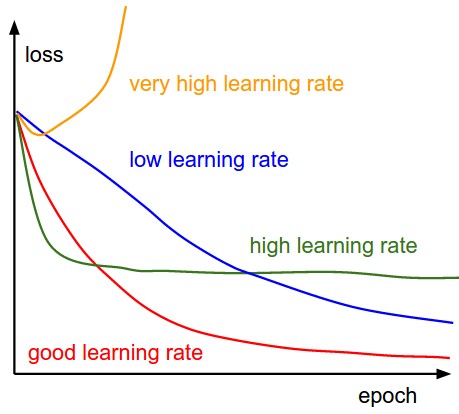
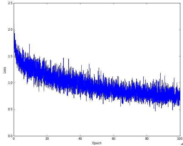Left: A cartoon depicting the effects of different learning rates. With low learning rates the improvements will be linear. With high learning rates they will start to look more exponential. Higher learning rates will decay the loss faster, but they get stuck at worse values of loss (green line). This is because there is too much “energy” in the optimization and the parameters are bouncing around chaotically, unable to settle in a nice spot in the optimization landscape. Right: An example of a typical loss function over time, while training a small network on CIFAR-10 dataset. This loss function looks reasonable (it might indicate a slightly too small learning rate based on its speed of decay, but it’s hard to say), and also indicates that the batch size might be a little too low (since the cost is a little too noisy).

왼쪽: 학습률이 다를 때의 효과를 그린 개념도. 학습률이 낮으면 개선이 선형에 가깝다. 학습률이 높으면 좀 더 지수적인 모양이 되기 시작한다. 학습률이 높을수록 손실이 더 빨리 떨어지지만 더 나쁜 손실 값에서 멈춰버린다(초록색 선). 최적화에 “에너지”가 너무 많아 매개변수들이 어지럽게 튀어 다니느라 최적화 지형의 좋은 자리에 내려앉지 못하기 때문이다. 오른쪽: CIFAR-10 데이터셋으로 작은 신경망을 학습시킬 때 나온, 시간에 따른 전형적인 손실 함수의 예. 이 손실 함수는 그럭저럭 괜찮아 보이며(떨어지는 속도로 보아 학습률이 살짝 작을 수도 있지만 단정하기는 어렵다), 비용이 조금 지나치게 들쭉날쭉한 것으로 보아 배치 크기가 조금 작을 수도 있음을 시사한다.

The amount of “wiggle” in the loss is related to the batch size. When the batch size is 1, the wiggle will be relatively high. When the batch size is the full dataset, the wiggle will be minimal because every gradient update should be improving the loss function monotonically (unless the learning rate is set too high).

손실이 “구불거리는” 정도는 배치 크기와 관련이 있다. 배치 크기가 1이면 구불거림이 비교적 크다. 배치 크기가 데이터셋 전체이면 구불거림이 최소가 되는데, (학습률을 너무 크게 잡지 않은 한) 기울기 갱신 하나하나가 손실 함수를 단조적으로 개선해야 하기 때문이다.

Some people prefer to plot their loss functions in the log domain. Since learning progress generally takes an exponential form shape, the plot appears as a slightly more interpretable straight line, rather than a hockey stick. Additionally, if multiple cross-validated models are plotted on the same loss graph, the differences between them become more apparent.

손실 함수를 로그 축에 그리기를 선호하는 사람들도 있다. 학습의 진행은 대체로 지수적인 형태를 띠므로, 로그 축에 그리면 하키 스틱 모양 대신 조금 더 읽기 쉬운 직선으로 나타난다. 게다가 교차 검증한 모델 여럿을 같은 손실 그래프에 겹쳐 그리면 그 차이가 더 뚜렷해진다.

Sometimes loss functions can look funny lossfunctions.tumblr.com.

손실 함수가 우스꽝스러운 모양이 될 때도 있다. lossfunctions.tumblr.com을 보라.

Train/Val accuracy

The second important quantity to track while training a classifier is the validation/training accuracy. This plot can give you valuable insights into the amount of overfitting in your model:

분류기를 학습시키는 동안 추적해야 할 두 번째로 중요한 양은 검증 정확도와 학습 정확도다. 이 그래프는 모델이 얼마나 과적합했는지에 대한 값진 통찰을 준다.

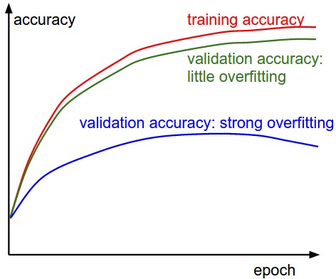The gap between the training and validation accuracy indicates the amount of overfitting. Two possible cases are shown in the diagram on the left. The blue validation error curve shows very small validation accuracy compared to the training accuracy, indicating strong overfitting (note, it’s possible for the validation accuracy to even start to go down after some point). When you see this in practice you probably want to increase regularization (stronger L2 weight penalty, more dropout, etc.) or collect more data. The other possible case is when the validation accuracy tracks the training accuracy fairly well. This case indicates that your model capacity is not high enough: make the model larger by increasing the number of parameters.

학습 정확도와 검증 정확도 사이의 간격은 과적합의 정도를 말해준다. 왼쪽 그림에 가능한 두 경우가 나와 있다. 파란색 검증 오차 곡선은 학습 정확도에 비해 검증 정확도가 매우 낮아 강한 과적합을 나타낸다(어느 시점 이후로는 검증 정확도가 아예 떨어지기 시작할 수도 있다). 실제로 이런 모습을 보면 정규화를 키우거나(더 강한 L2 가중치 벌점, 더 많은 dropout 등) 데이터를 더 모으고 싶어질 것이다. 다른 가능한 경우는 검증 정확도가 학습 정확도를 꽤 잘 따라가는 경우다. 이는 모델의 수용력이 충분히 높지 않다는 뜻이다. 매개변수 수를 늘려 모델을 더 크게 만들자.

Ratio of weights:updates

The last quantity you might want to track is the ratio of the update magnitudes to the value magnitudes. Note: updates, not the raw gradients (e.g. in vanilla sgd this would be the gradient multiplied by the learning rate). You might want to evaluate and track this ratio for every set of parameters independently. A rough heuristic is that this ratio should be somewhere around 1e-3. If it is lower than this then the learning rate might be too low. If it is higher then the learning rate is likely too high. Here is a specific example:

마지막으로 추적해볼 만한 양은 갱신량의 크기와 값 자체의 크기의 비다. 주의할 것은 날것의 기울기가 아니라 갱신량이라는 점이다(예컨대 바닐라 SGD라면 기울기에 학습률을 곱한 값이다). 이 비는 매개변수 묶음마다 따로 계산해 추적하는 편이 좋다. 대략적인 어림법으로 이 비는 1e-3 언저리여야 한다. 이보다 낮으면 학습률이 너무 낮은 것일 수 있다. 이보다 높으면 학습률이 너무 높을 가능성이 크다. 구체적인 예를 들면 다음과 같다.

# assume parameter vector W and its gradient vector dW
param_scale = np.linalg.norm(W.ravel())
update = -learning_rate*dW # simple SGD update
update_scale = np.linalg.norm(update.ravel())
W += update # the actual update
print update_scale / param_scale # want ~1e-3

Instead of tracking the min or the max, some people prefer to compute and track the norm of the gradients and their updates instead. These metrics are usually correlated and often give approximately the same results.

최솟값이나 최댓값을 추적하는 대신 기울기와 갱신량의 노름을 계산해 추적하기를 선호하는 사람들도 있다. 이 지표들은 대개 서로 상관이 있어서 대체로 비슷한 결과를 준다.

Activation / Gradient distributions per layer

An incorrect initialization can slow down or even completely stall the learning process. Luckily, this issue can be diagnosed relatively easily. One way to do so is to plot activation/gradient histograms for all layers of the network. Intuitively, it is not a good sign to see any strange distributions - e.g. with tanh neurons we would like to see a distribution of neuron activations between the full range of [-1,1], instead of seeing all neurons outputting zero, or all neurons being completely saturated at either -1 or 1.

초기화가 잘못되면 학습이 느려지거나 아예 완전히 멈춰버릴 수 있다. 다행히 이 문제는 비교적 쉽게 진단할 수 있다. 한 가지 방법은 신경망의 모든 층에 대해 활성값과 기울기의 히스토그램을 그려보는 것이다. 직관적으로, 이상한 분포가 보이는 것은 좋은 신호가 아니다. 예컨대 tanh 뉴런이라면 뉴런 활성값이 [-1,1] 구간 전체에 퍼진 분포를 보고 싶지, 모든 뉴런이 0을 내놓거나 모든 뉴런이 -1이나 1에서 완전히 포화한 모습을 보고 싶지는 않다.

First-layer Visualizations

Lastly, when one is working with image pixels it can be helpful and satisfying to plot the first-layer features visually:

마지막으로, 이미지 픽셀을 다루고 있다면 첫 번째 층의 특징을 눈으로 그려보는 것이 도움이 되고 보람도 있다.

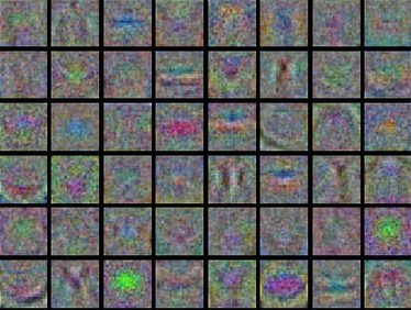
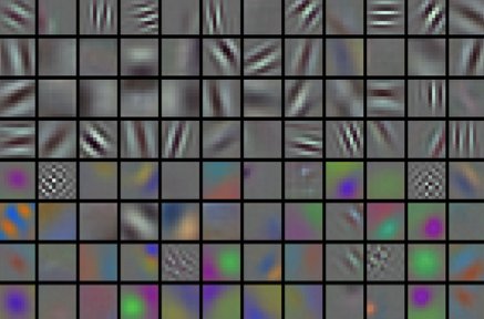Examples of visualized weights for the first layer of a neural network. Left: Noisy features indicate could be a symptom: Unconverged network, improperly set learning rate, very low weight regularization penalty. Right: Nice, smooth, clean and diverse features are a good indication that the training is proceeding well.

신경망 첫 번째 층의 가중치를 시각화한 예. 왼쪽: 잡음이 많은 특징은 신경망이 아직 수렴하지 않았거나, 학습률이 잘못 설정되었거나, 가중치 정규화 벌점이 지나치게 낮다는 징후일 수 있다. 오른쪽: 매끄럽고 깔끔하며 다양한 특징은 학습이 잘 진행되고 있다는 좋은 신호다.

Parameter updates

Once the analytic gradient is computed with backpropagation, the gradients are used to perform a parameter update. There are several approaches for performing the update, which we discuss next.

역전파로 해석적 기울기를 계산하고 나면 그 기울기를 써서 매개변수를 갱신한다. 갱신을 수행하는 방식에는 여러 접근이 있으며 이제 그것들을 살펴본다.

We note that optimization for deep networks is currently a very active area of research. In this section we highlight some established and common techniques you may see in practice, briefly describe their intuition, but leave a detailed analysis outside of the scope of the class. We provide some further pointers for an interested reader.

깊은 신경망의 최적화는 현재 매우 활발한 연구 분야라는 점을 짚어둔다. 이 절에서는 실전에서 마주칠 만한, 어느 정도 자리 잡은 흔한 기법 몇 가지를 짚고 그 직관을 짧게 설명하되, 자세한 분석은 이 수업의 범위 밖으로 둔다. 관심 있는 독자를 위해 더 볼거리를 몇 개 남겨둔다.

SGD and bells and whistles

Vanilla update. The simplest form of update is to change the parameters along the negative gradient direction (since the gradient indicates the direction of increase, but we usually wish to minimize a loss function). Assuming a vector of parameters x and the gradient dx, the simplest update has the form:

바닐라 갱신. 가장 단순한 형태의 갱신은 매개변수를 기울기의 반대 방향으로 옮기는 것이다(기울기는 증가하는 방향을 가리키는데 우리는 보통 손실 함수를 최소화하고 싶기 때문이다). 매개변수 벡터 x와 기울기 dx가 있다고 하면 가장 단순한 갱신은 다음과 같은 형태다.

# Vanilla update
x += - learning_rate * dx

where learning_rate is a hyperparameter - a fixed constant. When evaluated on the full dataset, and when the learning rate is low enough, this is guaranteed to make non-negative progress on the loss function.

여기서 learning_rate는 하이퍼파라미터, 곧 고정된 상수다. 데이터셋 전체에 대해 계산하고 학습률이 충분히 낮다면, 이 갱신은 손실 함수에서 음이 아닌 진전을 낸다는 것이 보장된다.

Momentum update is another approach that almost always enjoys better converge rates on deep networks. This update can be motivated from a physical perspective of the optimization problem. In particular, the loss can be interpreted as the height of a hilly terrain (and therefore also to the potential energy since \(U = mgh\) and therefore \(U \propto h\) ). Initializing the parameters with random numbers is equivalent to setting a particle with zero initial velocity at some location. The optimization process can then be seen as equivalent to the process of simulating the parameter vector (i.e. a particle) as rolling on the landscape.

Momentum 갱신은 깊은 신경망에서 거의 언제나 더 나은 수렴 속도를 내는 또 다른 접근이다. 이 갱신은 최적화 문제를 물리적으로 바라보는 관점에서 이끌어낼 수 있다. 구체적으로, 손실을 언덕진 지형의 높이로 볼 수 있다(\(U = mgh\)이므로 위치 에너지로도 볼 수 있다. 즉 \(U \propto h\)다). 매개변수를 난수로 초기화하는 것은 입자를 어떤 위치에 초기 속도 0으로 놓아두는 것과 같다. 그러면 최적화 과정은 매개변수 벡터, 곧 입자가 그 지형 위를 굴러가는 것을 시뮬레이션하는 과정과 같아진다.

Since the force on the particle is related to the gradient of potential energy (i.e. \(F = - \nabla U\) ), the force felt by the particle is precisely the (negative) gradient of the loss function. Moreover, \(F = ma\) so the (negative) gradient is in this view proportional to the acceleration of the particle. Note that this is different from the SGD update shown above, where the gradient directly integrates the position. Instead, the physics view suggests an update in which the gradient only directly influences the velocity, which in turn has an effect on the position:

입자에 작용하는 힘은 위치 에너지의 기울기와 관련되므로(\(F = - \nabla U\)), 입자가 느끼는 힘은 정확히 손실 함수의 (음의) 기울기다. 또 \(F = ma\)이므로 이 관점에서 (음의) 기울기는 입자의 가속도에 비례한다. 이것은 위에서 본 SGD 갱신과 다르다는 점에 주목하자. SGD에서는 기울기가 위치에 곧바로 적분되어 들어갔다. 반면 물리적 관점은 기울기가 속도에만 직접 영향을 주고 그 속도가 다시 위치에 영향을 주는 형태의 갱신을 제안한다.

# Momentum update
v = mu * v - learning_rate * dx # integrate velocity
x += v # integrate position

Here we see an introduction of a v variable that is initialized at zero, and an additional hyperparameter (mu). As an unfortunate misnomer, this variable is in optimization referred to as momentum (its typical value is about 0.9), but its physical meaning is more consistent with the coefficient of friction. Effectively, this variable damps the velocity and reduces the kinetic energy of the system, or otherwise the particle would never come to a stop at the bottom of a hill. When cross-validated, this parameter is usually set to values such as [0.5, 0.9, 0.95, 0.99]. Similar to annealing schedules for learning rates (discussed later, below), optimization can sometimes benefit a little from momentum schedules, where the momentum is increased in later stages of learning. A typical setting is to start with momentum of about 0.5 and anneal it to 0.99 or so over multiple epochs.

여기서 0으로 초기화되는 변수 v와 하이퍼파라미터 하나(mu)가 새로 등장한다. 안타깝게도 잘못 붙은 이름인데, 최적화 분야에서 이 변수를 momentum이라고 부르지만(전형적인 값은 0.9 정도다) 물리적 의미로는 마찰 계수 쪽에 더 가깝다. 실제로 이 변수는 속도를 감쇠시켜 계의 운동 에너지를 줄인다. 그러지 않으면 입자가 언덕 바닥에서 결코 멈추지 못할 것이다. 교차 검증할 때 이 매개변수는 보통 [0.5, 0.9, 0.95, 0.99] 같은 값으로 잡는다. (뒤에서 다룰) 학습률 담금질 일정과 비슷하게, momentum 일정으로 최적화가 조금 이득을 보는 경우도 있다. momentum 일정이란 학습 후반으로 갈수록 momentum을 키우는 것이다. 전형적인 설정은 momentum을 0.5 정도로 시작해 여러 epoch에 걸쳐 0.99쯤까지 담금질하는 것이다.

With Momentum update, the parameter vector will build up velocity in any direction that has consistent gradient.

Momentum 갱신을 쓰면 매개변수 벡터는 기울기가 일관되게 유지되는 방향이라면 어느 방향으로든 속도를 쌓아간다.

Nesterov Momentum is a slightly different version of the momentum update that has recently been gaining popularity. It enjoys stronger theoretical converge guarantees for convex functions and in practice it also consistenly works slightly better than standard momentum.

Nesterov momentum은 momentum 갱신을 조금 변형한 것으로 최근 인기를 얻고 있다. 볼록 함수에 대해 더 강한 이론적 수렴 보장을 가지며, 실전에서도 표준 momentum보다 꾸준히 조금 더 잘 동작한다.

The core idea behind Nesterov momentum is that when the current parameter vector is at some position x, then looking at the momentum update above, we know that the momentum term alone (i.e. ignoring the second term with the gradient) is about to nudge the parameter vector by mu * v. Therefore, if we are about to compute the gradient, we can treat the future approximate position x + mu * v as a “lookahead” - this is a point in the vicinity of where we are soon going to end up. Hence, it makes sense to compute the gradient at x + mu * v instead of at the “old/stale” position x.

Nesterov momentum의 핵심 착상은 이렇다. 현재 매개변수 벡터가 위치 x에 있다고 하자. 위의 momentum 갱신을 보면 momentum 항 하나만으로도(즉 기울기가 들어간 두 번째 항을 무시하더라도) 매개변수 벡터가 곧 mu * v만큼 밀려나리라는 것을 우리는 이미 알고 있다. 그러므로 기울기를 계산하려는 참이라면, 앞으로 도착할 대략적인 위치 x + mu * v를 “미리 내다본” 지점으로 취급할 수 있다. 곧 우리가 도착하게 될 곳 근처의 한 점이다. 따라서 “낡은” 위치 x 대신 x + mu * v에서 기울기를 계산하는 것이 이치에 맞다.

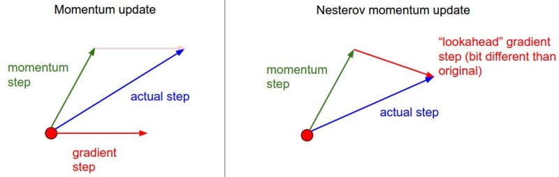Nesterov momentum. Instead of evaluating gradient at the current position (red circle), we know that our momentum is about to carry us to the tip of the green arrow. With Nesterov momentum we therefore instead evaluate the gradient at this “looked-ahead” position.

Nesterov momentum. 현재 위치(빨간 원)에서 기울기를 계산하는 대신, momentum이 우리를 초록 화살표 끝으로 곧 데려가리라는 것을 우리는 알고 있다. 그래서 Nesterov momentum에서는 이 “미리 내다본” 위치에서 기울기를 계산한다.

That is, in a slightly awkward notation, we would like to do the following:

즉 조금 어색한 표기를 쓰자면 우리가 하고 싶은 것은 다음과 같다.

x_ahead = x + mu * v
# evaluate dx_ahead (the gradient at x_ahead instead of at x)
v = mu * v - learning_rate * dx_ahead
x += v

However, in practice people prefer to express the update to look as similar to vanilla SGD or to the previous momentum update as possible. This is possible to achieve by manipulating the update above with a variable transform x_ahead = x + mu * v, and then expressing the update in terms of x_ahead instead of x. That is, the parameter vector we are actually storing is always the ahead version. The equations in terms of x_ahead (but renaming it back to x) then become:

그런데 실전에서는 갱신 식이 바닐라 SGD나 앞의 momentum 갱신과 최대한 비슷한 모습이기를 사람들이 선호한다. 위 갱신에 x_ahead = x + mu * v라는 변수 변환을 적용해 x 대신 x_ahead로 갱신을 다시 쓰면 그렇게 만들 수 있다. 즉 실제로 저장하고 있는 매개변수 벡터는 언제나 앞서 내다본 쪽이다. x_ahead로 쓴 식은(그리고 그 이름을 다시 x로 되돌리면) 다음과 같아진다.

역주. 변수 변환이 저 식을 어떻게 만드는지 한 번 따라가 두면 코드가 낯설지 않다. 앞의 식은 실제 위치 \(x_t\)와 앞서 내다본 위치 \(\tilde{x}_t = x_t + \mu v_t\) 두 가지를 오간다. 저장하는 값을 \(\tilde{x}\) 쪽으로 통일해보자. 속도 갱신은 그대로 \(v_{t+1} = \mu v_t - \eta \nabla f(\tilde{x}_t)\)이고 위치 갱신은 \(x_{t+1} = x_t + v_{t+1}\)인데, 여기에 \(x_t = \tilde{x}_t - \mu v_t\)를 넣으면

\[\tilde{x}_{t+1} = x_{t+1} + \mu v_{t+1} = \tilde{x}_t - \mu v_t + (1 + \mu) v_{t+1}\]

이 된다. 이름을 다시 \(x\)로 되돌린 것이 코드의 x += -mu * v_prev + (1 + mu) * v이고, \(v_t\)를 미리 챙겨둔 것이 v_prev다. 요점은 기울기를 재는 지점이 언제나 앞서 내다본 위치라는 것이며, 그래서 이 형태에서는 dx를 평소처럼 현재 저장된 x에서 계산해도 Nesterov가 된다.

v_prev = v # back this up
v = mu * v - learning_rate * dx # velocity update stays the same
x += -mu * v_prev + (1 + mu) * v # position update changes form

We recommend this further reading to understand the source of these equations and the mathematical formulation of Nesterov’s Accelerated Momentum (NAG):

이 식들이 어디서 나왔는지, Nesterov 가속 momentum(NAG)의 수학적 정식화가 무엇인지 이해하려면 다음 자료를 더 읽어보기를 권한다.

• Advances in optimizing Recurrent Networks by Yoshua Bengio, Section 3.5.
• Ilya Sutskever’s thesis (pdf) contains a longer exposition of the topic in section 7.2

• Yoshua Bengio의 Advances in optimizing Recurrent Networks 3.5절.
• Ilya Sutskever의 학위 논문(pdf) 7.2절에 이 주제가 더 길게 설명되어 있다

Annealing the learning rate

In training deep networks, it is usually helpful to anneal the learning rate over time. Good intuition to have in mind is that with a high learning rate, the system contains too much kinetic energy and the parameter vector bounces around chaotically, unable to settle down into deeper, but narrower parts of the loss function. Knowing when to decay the learning rate can be tricky: Decay it slowly and you’ll be wasting computation bouncing around chaotically with little improvement for a long time. But decay it too aggressively and the system will cool too quickly, unable to reach the best position it can. There are three common types of implementing the learning rate decay:

깊은 신경망을 학습시킬 때는 시간이 지남에 따라 학습률을 담금질하는 것이 대개 도움이 된다. 염두에 둘 좋은 직관은 이렇다. 학습률이 높으면 계의 운동 에너지가 지나치게 커서 매개변수 벡터가 어지럽게 튀어 다니고, 손실 함수의 더 깊지만 좁은 골짜기에 내려앉지 못한다. 언제 학습률을 감쇠시킬지 판단하기는 까다롭다. 천천히 감쇠시키면 오랫동안 별 개선 없이 어지럽게 튀어 다니며 계산을 낭비하게 된다. 그렇다고 너무 공격적으로 감쇠시키면 계가 너무 빨리 식어버려 도달할 수 있는 가장 좋은 자리에 이르지 못한다. 학습률 감쇠를 구현하는 흔한 방식은 세 가지다.

• Step decay: Reduce the learning rate by some factor every few epochs. Typical values might be reducing the learning rate by a half every 5 epochs, or by 0.1 every 20 epochs. These numbers depend heavily on the type of problem and the model. One heuristic you may see in practice is to watch the validation error while training with a fixed learning rate, and reduce the learning rate by a constant (e.g. 0.5) whenever the validation error stops improving.
• Exponential decay. has the mathematical form \(\alpha = \alpha_0 e^{-k t}\), where \(\alpha_0, k\) are hyperparameters and \(t\) is the iteration number (but you can also use units of epochs).
• 1/t decay has the mathematical form \(\alpha = \alpha_0 / (1 + k t )\) where \(a_0, k\) are hyperparameters and \(t\) is the iteration number.

• 계단 감쇠(step decay): 몇 epoch마다 학습률을 어떤 비율로 줄인다. 전형적으로는 5 epoch마다 학습률을 절반으로, 또는 20 epoch마다 0.1배로 줄이는 정도다. 이 수치들은 문제의 종류와 모델에 크게 좌우된다. 실전에서 볼 수 있는 어림법 하나는, 학습률을 고정한 채 학습하면서 검증 오차를 지켜보다가 검증 오차가 더 이상 좋아지지 않을 때마다 학습률에 상수(예컨대 0.5)를 곱해 줄이는 것이다.
• 지수 감쇠. \(\alpha = \alpha_0 e^{-k t}\)라는 수식 형태를 갖는다. 여기서 \(\alpha_0, k\)는 하이퍼파라미터이고 \(t\)는 반복 횟수다(epoch 단위를 써도 된다).
• 1/t 감쇠는 \(\alpha = \alpha_0 / (1 + k t )\)라는 수식 형태를 갖는다. 여기서 \(a_0, k\)는 하이퍼파라미터이고 \(t\)는 반복 횟수다.

In practice, we find that the step decay is slightly preferable because the hyperparameters it involves (the fraction of decay and the step timings in units of epochs) are more interpretable than the hyperparameter \(k\). Lastly, if you can afford the computational budget, err on the side of slower decay and train for a longer time.

실전에서는 계단 감쇠가 약간 더 낫다고 본다. 계단 감쇠에 들어가는 하이퍼파라미터(감쇠 비율과 epoch 단위로 표현한 감쇠 시점)가 하이퍼파라미터 \(k\)보다 해석하기 쉽기 때문이다. 마지막으로, 계산 예산에 여유가 있다면 감쇠를 더 느리게 하는 쪽으로 기울이고 더 오래 학습시켜라.

Second order methods

A second, popular group of methods for optimization in context of deep learning is based on Newton’s method, which iterates the following update:

\[x \leftarrow x - [H f(x)]^{-1} \nabla f(x)\]

딥러닝 맥락에서 두 번째로 인기 있는 최적화 방법 무리는 뉴턴 방법에 기반하며, 다음 갱신을 반복한다.

Here, \(H f(x)\) is the Hessian matrix, which is a square matrix of second-order partial derivatives of the function. The term \(\nabla f(x)\) is the gradient vector, as seen in Gradient Descent. Intuitively, the Hessian describes the local curvature of the loss function, which allows us to perform a more efficient update. In particular, multiplying by the inverse Hessian leads the optimization to take more aggressive steps in directions of shallow curvature and shorter steps in directions of steep curvature. Note, crucially, the absence of any learning rate hyperparameters in the update formula, which the proponents of these methods cite this as a large advantage over first-order methods.

여기서 \(H f(x)\)는 헤세 행렬로, 함수의 2차 편미분으로 이루어진 정사각 행렬이다. \(\nabla f(x)\) 항은 경사 하강법에서 본 기울기 벡터다. 직관적으로 헤세 행렬은 손실 함수의 국소적인 곡률을 나타내며, 덕분에 더 효율적인 갱신을 할 수 있다. 구체적으로 헤세 역행렬을 곱하면 최적화가 곡률이 완만한 방향으로는 더 과감하게, 곡률이 가파른 방향으로는 더 짧게 나아가게 된다. 결정적으로 이 갱신 식에는 학습률 하이퍼파라미터가 아예 없다는 점에 주목하자. 이 방법들을 지지하는 이들은 이 점을 1차 방법에 대한 큰 이점으로 꼽는다.

However, the update above is impractical for most deep learning applications because computing (and inverting) the Hessian in its explicit form is a very costly process in both space and time. For instance, a Neural Network with one million parameters would have a Hessian matrix of size [1,000,000 x 1,000,000], occupying approximately 3725 gigabytes of RAM. Hence, a large variety of quasi-Newton methods have been developed that seek to approximate the inverse Hessian. Among these, the most popular is L-BFGS, which uses the information in the gradients over time to form the approximation implicitly (i.e. the full matrix is never computed).

그러나 위 갱신은 대부분의 딥러닝 응용에서 비현실적이다. 헤세 행렬을 명시적으로 계산하고 그 역행렬을 구하는 일이 공간과 시간 양쪽에서 매우 비싸기 때문이다. 예컨대 매개변수가 백만 개인 신경망의 헤세 행렬은 [1,000,000 x 1,000,000] 크기이고 대략 3725기가바이트의 RAM을 차지한다. 그래서 헤세 역행렬을 근사하려는 준-뉴턴 방법들이 다양하게 개발되었다. 그중 가장 인기 있는 것은 L-BFGS로, 시간에 걸쳐 쌓인 기울기 정보를 써서 근사를 암묵적으로 만들어낸다(즉 전체 행렬을 한 번도 계산하지 않는다).

However, even after we eliminate the memory concerns, a large downside of a naive application of L-BFGS is that it must be computed over the entire training set, which could contain millions of examples. Unlike mini-batch SGD, getting L-BFGS to work on mini-batches is more tricky and an active area of research.

그런데 메모리 문제를 없애더라도 L-BFGS를 그대로 갖다 쓰는 데는 큰 단점이 남는다. 학습 집합 전체에 대해 계산해야 하는데 그 안에는 예제가 수백만 개 있을 수 있다는 점이다. mini-batch SGD와 달리 L-BFGS를 mini-batch에서 동작하게 만드는 것은 훨씬 까다로우며 활발한 연구 분야다.

In practice, it is currently not common to see L-BFGS or similar second-order methods applied to large-scale Deep Learning and Convolutional Neural Networks. Instead, SGD variants based on (Nesterov’s) momentum are more standard because they are simpler and scale more easily.

실전에서는 대규모 딥러닝과 합성곱 신경망에 L-BFGS 같은 2차 방법을 적용하는 경우를 지금은 보기 어렵다. 대신 (Nesterov) momentum에 기반한 SGD 변형들이 더 표준적인데, 더 간단하고 규모를 키우기도 더 쉽기 때문이다.

Additional references:

더 볼 자료는 다음과 같다.

• Large Scale Distributed Deep Networks is a paper from the Google Brain team, comparing L-BFGS and SGD variants in large-scale distributed optimization.
• SFO algorithm strives to combine the advantages of SGD with advantages of L-BFGS.

• Large Scale Distributed Deep Networks는 Google Brain 팀의 논문으로, 대규모 분산 최적화에서 L-BFGS와 SGD 변형들을 비교한다.
• SFO 알고리즘은 SGD의 장점과 L-BFGS의 장점을 결합하려 한다.

Per-parameter adaptive learning rate methods

All previous approaches we’ve discussed so far manipulated the learning rate globally and equally for all parameters. Tuning the learning rates is an expensive process, so much work has gone into devising methods that can adaptively tune the learning rates, and even do so per parameter. Many of these methods may still require other hyperparameter settings, but the argument is that they are well-behaved for a broader range of hyperparameter values than the raw learning rate. In this section we highlight some common adaptive methods you may encounter in practice:

지금까지 논한 모든 접근은 학습률을 전역적으로, 그리고 모든 매개변수에 똑같이 다뤘다. 학습률을 조율하는 일은 비싼 과정이므로, 학습률을 적응적으로, 나아가 매개변수마다 따로 조율하는 방법을 고안하는 데 많은 노력이 들어갔다. 이런 방법들도 여전히 다른 하이퍼파라미터 설정을 요구하는 경우가 많지만, 날것의 학습률보다 훨씬 넓은 범위의 하이퍼파라미터 값에서 무난하게 동작한다는 것이 그 논지다. 이 절에서는 실전에서 마주칠 만한 흔한 적응적 방법 몇 가지를 짚는다.

Adagrad is an adaptive learning rate method originally proposed by Duchi et al..

Adagrad는 Duchi 등이 처음 제안한 적응적 학습률 방법이다.

# Assume the gradient dx and parameter vector x
cache += dx**2
x += - learning_rate * dx / (np.sqrt(cache) + eps)

Notice that the variable cache has size equal to the size of the gradient, and keeps track of per-parameter sum of squared gradients. This is then used to normalize the parameter update step, element-wise. Notice that the weights that receive high gradients will have their effective learning rate reduced, while weights that receive small or infrequent updates will have their effective learning rate increased. Amusingly, the square root operation turns out to be very important and without it the algorithm performs much worse. The smoothing term eps (usually set somewhere in range from 1e-4 to 1e-8) avoids division by zero. A downside of Adagrad is that in case of Deep Learning, the monotonic learning rate usually proves too aggressive and stops learning too early.

변수 cache의 크기는 기울기와 같으며, 매개변수마다 기울기 제곱의 합을 누적해 기록한다는 점에 주목하자. 그리고 이것을 써서 매개변수 갱신 스텝을 원소별로 정규화(normalization)한다. 큰 기울기를 받은 가중치는 실효 학습률이 줄어들고, 작거나 드문 갱신만 받은 가중치는 실효 학습률이 커진다는 점에 주목하자. 재미있게도 제곱근 연산이 매우 중요한 것으로 드러났으며, 이것이 없으면 알고리즘 성능이 훨씬 나빠진다. 매끄럽게 만드는 항 eps(보통 1e-4에서 1e-8 범위로 잡는다)는 0으로 나누는 것을 막는다. Adagrad의 단점은, 딥러닝에서는 학습률이 단조적으로 줄어들기만 하는 것이 대개 지나치게 공격적이어서 학습이 너무 일찍 멈춰버린다는 점이다.

역주. 제곱근이 왜 그렇게 중요한지는 원문이 “재미있게도”라고만 하고 넘어가는데, cache의 규모를 따져보면 풀린다. cache는 기울기의 제곱을 누적한 값이라 크기가 기울기의 제곱 규모다. 여기에 제곱근을 씌우면 분모가 기울기와 같은 규모가 되어 dx / sqrt(cache)는 대략 \(-1\)과 \(1\) 사이의 무차원 양이 되고, 그래서 한 스텝의 크기가 기울기가 크든 작든 learning_rate 언저리로 묶인다. 제곱근을 빼고 dx / cache로 쓰면 이 비가 대략 \(1/g\)가 되어, 기울기가 작은 매개변수일수록 갱신량이 오히려 발산하듯 커진다. 기울기 크기에 맞춰 스텝을 고르게 만들려던 장치가 정반대로 뒤집히는 셈이다.

RMSprop. RMSprop is a very effective, but currently unpublished adaptive learning rate method. Amusingly, everyone who uses this method in their work currently cites slide 29 of Lecture 6 of Geoff Hinton’s Coursera class. The RMSProp update adjusts the Adagrad method in a very simple way in an attempt to reduce its aggressive, monotonically decreasing learning rate. In particular, it uses a moving average of squared gradients instead, giving:

RMSprop. RMSprop은 매우 효과적이지만 현재까지 출판되지 않은 적응적 학습률 방법이다. 재미있게도 이 방법을 연구에 쓰는 사람들은 모두 Geoff Hinton의 Coursera 강의 6강 29번 슬라이드를 인용한다. RMSProp 갱신은 Adagrad의 공격적이고 단조적으로 감소하기만 하는 학습률을 누그러뜨리려고 아주 간단한 방식으로 Adagrad를 손본다. 구체적으로는 기울기 제곱의 이동 평균을 대신 쓰며, 식은 다음과 같다.

cache = decay_rate * cache + (1 - decay_rate) * dx**2
x += - learning_rate * dx / (np.sqrt(cache) + eps)

Here, decay_rate is a hyperparameter and typical values are [0.9, 0.99, 0.999]. Notice that the x+= update is identical to Adagrad, but the cache variable is a “leaky”. Hence, RMSProp still modulates the learning rate of each weight based on the magnitudes of its gradients, which has a beneficial equalizing effect, but unlike Adagrad the updates do not get monotonically smaller.

여기서 decay_rate는 하이퍼파라미터이고 전형적인 값은 [0.9, 0.99, 0.999]다. x+= 갱신은 Adagrad와 똑같지만 cache 변수가 “새는” 형태라는 점에 주목하자. 그래서 RMSProp도 여전히 각 가중치의 기울기 크기에 맞춰 학습률을 조절하며 이는 서로 다른 가중치를 고르게 만들어주는 이로운 효과를 내지만, Adagrad와 달리 갱신량이 단조적으로 작아지지는 않는다.

Adam. Adam is a recently proposed update that looks a bit like RMSProp with momentum. The (simplified) update looks as follows:

Adam. Adam은 최근 제안된 갱신 방식으로, momentum을 얹은 RMSProp과 조금 비슷한 모습이다. (단순화한) 갱신은 다음과 같다.

m = beta1*m + (1-beta1)*dx
v = beta2*v + (1-beta2)*(dx**2)
x += - learning_rate * m / (np.sqrt(v) + eps)

Notice that the update looks exactly as RMSProp update, except the “smooth” version of the gradient m is used instead of the raw (and perhaps noisy) gradient vector dx. Recommended values in the paper are eps = 1e-8, beta1 = 0.9, beta2 = 0.999. In practice Adam is currently recommended as the default algorithm to use, and often works slightly better than RMSProp. However, it is often also worth trying SGD+Nesterov Momentum as an alternative. The full Adam update also includes a bias correction mechanism, which compensates for the fact that in the first few time steps the vectors m,v are both initialized and therefore biased at zero, before they fully “warm up”. With the bias correction mechanism, the update looks as follows:

이 갱신이 RMSProp 갱신과 똑같이 생겼다는 점에 주목하자. 다만 날것의(그래서 잡음이 섞였을) 기울기 벡터 dx 대신 기울기를 “매끄럽게” 만든 m을 쓴다는 점만 다르다. 논문이 권하는 값은 eps = 1e-8, beta1 = 0.9, beta2 = 0.999다. 실전에서 Adam은 현재 기본으로 쓰기를 권하는 알고리즘이며 RMSProp보다 조금 더 잘 되는 경우가 많다. 다만 SGD+Nesterov momentum도 대안으로 시도해볼 만하다. 완전한 Adam 갱신에는 편향 보정(bias correction) 장치도 들어간다. 처음 몇 스텝 동안은 벡터 m과 v가 둘 다 0으로 초기화되어 있어 완전히 “예열”되기 전까지 0 쪽으로 편향되어 있는데, 편향 보정은 이를 바로잡는다. 편향 보정 장치까지 넣은 갱신은 다음과 같다.

역주. 편향 보정의 나눗셈 \(1 - \beta_1^t\)가 어디서 오는지는 m을 펼쳐보면 보인다. \(m_0 = 0\)에서 시작해 \(m_t = \beta_1 m_{t-1} + (1-\beta_1) g_t\)를 반복하면

\[m_t = (1-\beta_1) \sum_{i=1}^{t} \beta_1^{\,t-i} g_i\]

이고, 기울기의 기댓값이 대체로 \(E[g]\)로 일정하다고 보면 계수의 합이 \((1-\beta_1)(1 + \beta_1 + \cdots + \beta_1^{t-1}) = 1 - \beta_1^t\)이므로 \(E[m_t] \approx (1 - \beta_1^t) E[g]\)가 된다. 즉 초반의 m은 실제 기울기보다 작다. \(\beta_1 = 0.9\)이면 \(t=1\)에서 계수가 0.1이라 열 배 작고, v 쪽은 \(\beta_2 = 0.999\)라 \(t=1\)에서 천 배 작다. 보정을 빼먹으면 두 편향이 서로 상쇄되지 않아 학습 초반 몇 스텝의 갱신량이 오히려 부풀어 오른다. 분자는 0.1배인데 분모의 \(\sqrt{v}\)는 \(\sqrt{0.001} \approx 0.0316\)배라, 비율로는 세 배 넘게 커지기 때문이다. mt와 vt로 나누는 것은 이 편향을 걷어내 첫 스텝부터 갱신량이 제 크기를 갖게 하는 장치다.

# t is your iteration counter going from 1 to infinity
m = beta1*m + (1-beta1)*dx
mt = m / (1-beta1**t)
v = beta2*v + (1-beta2)*(dx**2)
vt = v / (1-beta2**t)
x += - learning_rate * mt / (np.sqrt(vt) + eps)

Note that the update is now a function of the iteration as well as the other parameters. We refer the reader to the paper for the details, or the course slides where this is expanded on.

이제 갱신이 다른 매개변수뿐 아니라 반복 횟수의 함수이기도 하다는 점에 주목하자. 자세한 내용은 논문이나, 이를 더 펼쳐 설명하는 수업 슬라이드를 참고하기 바란다.

Additional References:

더 볼 자료는 다음과 같다.

• Unit Tests for Stochastic Optimization proposes a series of tests as a standardized benchmark for stochastic optimization.

• Unit Tests for Stochastic Optimization은 확률적 최적화의 표준 벤치마크로 삼을 만한 일련의 테스트를 제안한다.

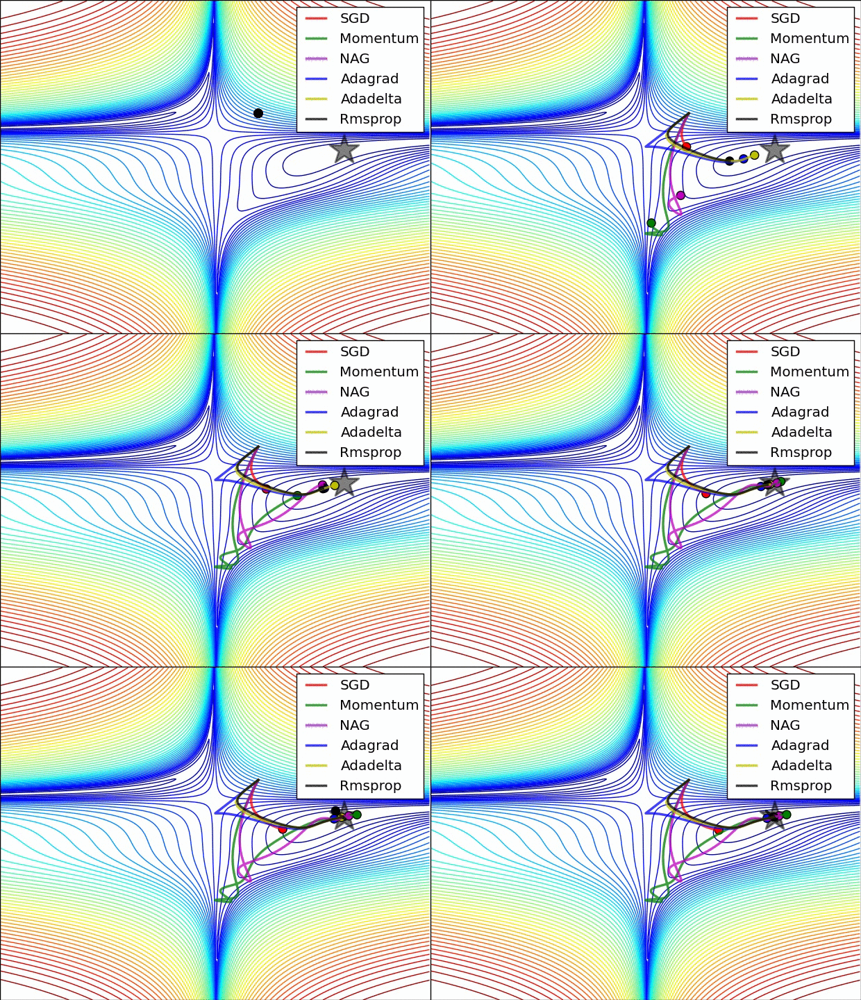
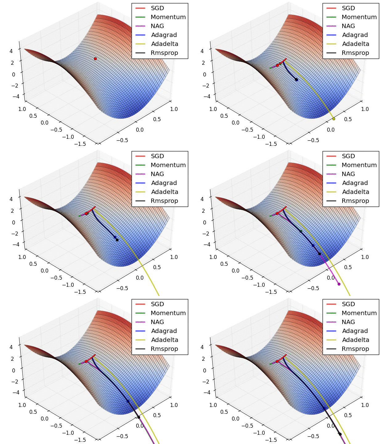Animations that may help your intuitions about the learning process dynamics. Left: Contours of a loss surface and time evolution of different optimization algorithms. Notice the “overshooting” behavior of momentum-based methods, which make the optimization look like a ball rolling down the hill. Right: A visualization of a saddle point in the optimization landscape, where the curvature along different dimension has different signs (one dimension curves up and another down). Notice that SGD has a very hard time breaking symmetry and gets stuck on the top. Conversely, algorithms such as RMSprop will see very low gradients in the saddle direction. Due to the denominator term in the RMSprop update, this will increase the effective learning rate along this direction, helping RMSProp proceed. Images credit: Alec Radford.

학습 과정의 동역학에 대한 직관을 돕는 애니메이션. 왼쪽: 손실 곡면의 등고선과 여러 최적화 알고리즘의 시간에 따른 궤적. momentum 계열 방법이 “지나쳐버리는” 모습에 주목하자. 최적화가 언덕을 굴러 내려가는 공처럼 보인다. 오른쪽: 최적화 지형에 있는 안장점의 시각화로, 차원마다 곡률의 부호가 다르다(한 차원은 위로 굽고 다른 차원은 아래로 굽는다). SGD가 대칭을 깨는 데 매우 애를 먹으며 꼭대기에 갇히는 것에 주목하자. 반대로 RMSprop 같은 알고리즘은 안장 방향에서 아주 작은 기울기를 보게 된다. RMSprop 갱신의 분모 항 덕분에 이 방향의 실효 학습률이 커지고, 그래서 RMSProp이 앞으로 나아갈 수 있다. 이미지 출처: Alec Radford.

보충: Adagrad와 RMSprop의 분모가 시간에 따라 어떻게 달라지는지 재어보기

두 규칙의 x += 줄은 글자 하나 다르지 않고, 갈리는 곳은 cache를 쌓는 방식 하나뿐이다. Adagrad는 제곱합을 그냥 더하기만 하고 RMSprop은 이동 평균이라 옛날 값이 새어 나간다. 이 차이가 실효 학습률 learning_rate / (sqrt(cache) + eps)에 무엇을 하는지, 궤적을 흉내 내지 말고 기울기 열을 직접 손으로 정해 재보자. 500스텝까지는 기울기가 10인 가파른 구간을 지나다가, 그 뒤로는 기울기가 0.1인 평평한 구간 — 바로 위 그림의 안장 방향 같은 곳 — 에 들어섰다고 하자.

import numpy as np

lr, eps, decay = 0.01, 1e-8, 0.99
STEPS, SWITCH = 2000, 500

# 500스텝까지는 가파른 구간(기울기 10), 그 뒤로는 평평한 구간(기울기 0.1)에 들어섰다고 하자
g = np.where(np.arange(STEPS) < SWITCH, 10.0, 0.1)

ada = rms = 0.0
eff = {}
for t in range(STEPS):
    ada += g[t] ** 2                              # Adagrad: 제곱합을 계속 누적한다
    rms = decay * rms + (1 - decay) * g[t] ** 2   # RMSprop: 새는 이동 평균
    eff[t + 1] = (lr / (np.sqrt(ada) + eps), lr / (np.sqrt(rms) + eps))

print(" 스텝   기울기   Adagrad 실효 학습률   RMSprop 실효 학습률")
for t in (1, 10, 100, 500, 501, 600, 1000, 2000):
    a, r = eff[t]
    print("%5d %8.2f %18.3e %21.3e" % (t, g[t - 1], a, r))

 스텝   기울기   Adagrad 실효 학습률   RMSprop 실효 학습률
    1    10.00          1.000e-03             1.000e-02
   10    10.00          3.162e-04             3.234e-03
  100    10.00          1.000e-04             1.256e-03
  500    10.00          4.472e-05             1.003e-03
  501     0.10          4.472e-05             1.008e-03
  600     0.10          4.472e-05             1.658e-03
 1000     0.10          4.472e-05             1.228e-02
 2000     0.10          4.471e-05             9.986e-02

가파른 구간에서는 둘 다 실효 학습률을 낮춘다. 여기까지는 의도한 대로다. 갈리는 곳은 501스텝 이후다. 기울기가 백분의 일로 줄었는데 Adagrad의 실효 학습률은 4.472e-05에서 꿈쩍도 하지 않는다. ada에 이미 쌓아둔 \(500 \times 10^2 = 50000\)이 그대로 남아 있고, 새로 더해지는 값은 \(0.1^2 = 0.01\)뿐이라 1500스텝을 더 가도 분모를 되돌리지 못하기 때문이다. 원문이 “학습률이 단조적으로 줄어들기만 하는 것이 지나치게 공격적이어서 학습이 너무 일찍 멈춘다”고 한 것이 바로 이 칸이다. 반면 RMSprop은 옛 기울기가 매 스텝 0.99배로 새어 나가므로 rms가 새 규모인 \(0.1^2\)을 향해 내려가고, 실효 학습률은 1.003e-03에서 9.986e-02로 백 배 회복한다. 2000스텝에서 두 값의 차이는 2200배가 넘는다. 바로 위 그림 설명이 “RMSprop 갱신의 분모 항 덕분에 이 방향의 실효 학습률이 커지고, 그래서 RMSProp이 앞으로 나아갈 수 있다”고 말한 것이 이 회복이다. Adagrad라면 같은 자리에서 그대로 굳는다.

Hyperparameter optimization

As we’ve seen, training Neural Networks can involve many hyperparameter settings. The most common hyperparameters in context of Neural Networks include:

지금까지 봤듯 신경망 학습에는 여러 하이퍼파라미터 설정이 얽힌다. 신경망 맥락에서 가장 흔한 하이퍼파라미터는 다음과 같다.

• the initial learning rate
• learning rate decay schedule (such as the decay constant)
• regularization strength (L2 penalty, dropout strength)

• 초기 학습률
• 학습률 감쇠 일정(감쇠 상수 같은 것)
• 정규화 세기(L2 벌점, dropout 세기)

But as we saw, there are many more relatively less sensitive hyperparameters, for example in per-parameter adaptive learning methods, the setting of momentum and its schedule, etc. In this section we describe some additional tips and tricks for performing the hyperparameter search:

그러나 앞에서 봤듯 상대적으로 덜 민감한 하이퍼파라미터가 훨씬 더 많다. 예컨대 매개변수별 적응적 학습률 방법의 설정값이나 momentum과 그 일정 같은 것들이다. 이 절에서는 하이퍼파라미터 탐색을 수행할 때 쓸 요령을 몇 가지 더 소개한다.

Implementation. Larger Neural Networks typically require a long time to train, so performing hyperparameter search can take many days/weeks. It is important to keep this in mind since it influences the design of your code base. One particular design is to have a worker that continuously samples random hyperparameters and performs the optimization. During the training, the worker will keep track of the validation performance after every epoch, and writes a model checkpoint (together with miscellaneous training statistics such as the loss over time) to a file, preferably on a shared file system. It is useful to include the validation performance directly in the filename, so that it is simple to inspect and sort the progress. Then there is a second program which we will call a master, which launches or kills workers across a computing cluster, and may additionally inspect the checkpoints written by workers and plot their training statistics, etc.

구현. 큰 신경망은 학습에 보통 오랜 시간이 걸리므로 하이퍼파라미터 탐색에 며칠에서 몇 주가 들 수 있다. 이것이 코드베이스 설계에 영향을 주므로 염두에 두는 것이 중요하다. 한 가지 설계는 하이퍼파라미터를 계속 무작위로 뽑아 최적화를 수행하는 작업자(worker)를 두는 것이다. 학습하는 동안 작업자는 매 epoch마다 검증 성능을 기록하고, 모델 체크포인트를 (시간에 따른 손실 같은 여러 학습 통계량과 함께) 파일로, 되도록이면 공유 파일 시스템에 쓴다. 검증 성능을 파일 이름에 직접 넣어두면 진행 상황을 살펴보고 정렬하기 쉬워 유용하다. 그리고 관리자(master)라고 부를 두 번째 프로그램을 둔다. 관리자는 계산 클러스터 전체에서 작업자를 띄우고 죽이며, 작업자들이 쓴 체크포인트를 살펴보고 학습 통계량을 그려보는 일 등을 추가로 할 수 있다.

Prefer one validation fold to cross-validation. In most cases a single validation set of respectable size substantially simplifies the code base, without the need for cross-validation with multiple folds. You’ll hear people say they “cross-validated” a parameter, but many times it is assumed that they still only used a single validation set.

교차 검증보다 검증 겹 하나를 선호한다. 대부분의 경우 적당한 크기의 검증 집합 하나만 두면 여러 겹으로 교차 검증할 필요가 없어 코드베이스가 크게 단순해진다. 어떤 매개변수를 “교차 검증했다”고 말하는 사람들을 보게 될 텐데, 많은 경우 그것도 검증 집합 하나만 썼다는 뜻으로 가정하면 된다.

Hyperparameter ranges. Search for hyperparameters on log scale. For example, a typical sampling of the learning rate would look as follows: learning_rate = 10 ** uniform(-6, 1). That is, we are generating a random number from a uniform distribution, but then raising it to the power of 10. The same strategy should be used for the regularization strength. Intuitively, this is because learning rate and regularization strength have multiplicative effects on the training dynamics. For example, a fixed change of adding 0.01 to a learning rate has huge effects on the dynamics if the learning rate is 0.001, but nearly no effect if the learning rate when it is 10. This is because the learning rate multiplies the computed gradient in the update. Therefore, it is much more natural to consider a range of learning rate multiplied or divided by some value, than a range of learning rate added or subtracted to by some value. Some parameters (e.g. dropout) are instead usually searched in the original scale (e.g. dropout = uniform(0,1)).

하이퍼파라미터 범위. 하이퍼파라미터는 로그 축에서 탐색한다. 예컨대 학습률의 전형적인 표집은 learning_rate = 10 ** uniform(-6, 1) 같은 모습이다. 즉 균등 분포에서 난수를 하나 뽑은 다음 그것을 10의 지수로 올린다. 정규화 세기에도 같은 전략을 써야 한다. 직관적으로 이렇게 하는 이유는 학습률과 정규화 세기가 학습 동역학에 곱셈으로 작용하기 때문이다. 예를 들어 학습률에 0.01을 더하는 고정된 변화는 학습률이 0.001일 때는 동역학에 큰 영향을 주지만 학습률이 10일 때는 사실상 아무 영향이 없다. 학습률이 갱신에서 계산된 기울기에 곱해지기 때문이다. 그러므로 학습률에 어떤 값을 더하거나 빼는 범위보다, 어떤 값을 곱하거나 나누는 범위를 생각하는 편이 훨씬 자연스럽다. 반면 어떤 매개변수(예컨대 dropout)는 보통 원래 축에서 탐색한다(예컨대 dropout = uniform(0,1)).

Prefer random search to grid search. As argued by Bergstra and Bengio in Random Search for Hyper-Parameter Optimization, “randomly chosen trials are more efficient for hyper-parameter optimization than trials on a grid”. As it turns out, this is also usually easier to implement.

격자 탐색보다 무작위 탐색을 선호한다. Bergstra와 Bengio가 Random Search for Hyper-Parameter Optimization에서 논했듯 “하이퍼파라미터 최적화에는 격자 위의 시도보다 무작위로 고른 시도가 더 효율적이다.” 게다가 구현하기도 대개 더 쉽다.

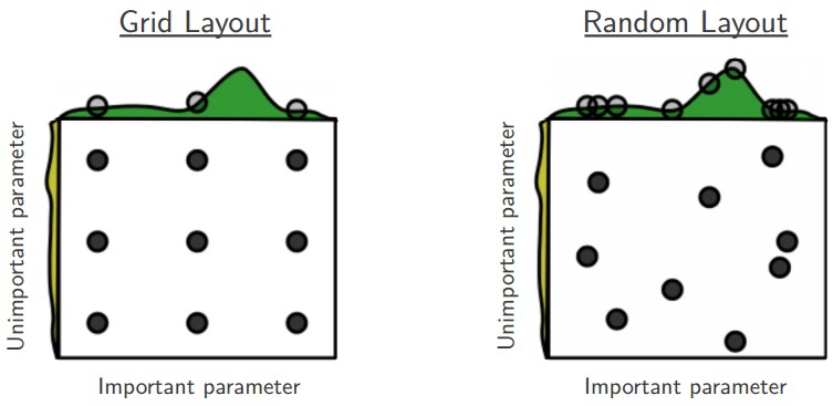Core illustration from Random Search for Hyper-Parameter Optimization by Bergstra and Bengio. It is very often the case that some of the hyperparameters matter much more than others (e.g. top hyperparam vs. left one in this figure). Performing random search rather than grid search allows you to much more precisely discover good values for the important ones.

Bergstra와 Bengio의 Random Search for Hyper-Parameter Optimization에 실린 핵심 그림. 어떤 하이퍼파라미터가 다른 것들보다 훨씬 더 중요한 경우가 매우 흔하다(예컨대 이 그림에서 위쪽 하이퍼파라미터와 왼쪽 하이퍼파라미터를 견줘보라). 격자 탐색 대신 무작위 탐색을 하면 중요한 하이퍼파라미터의 좋은 값을 훨씬 더 정밀하게 찾아낼 수 있다.

Careful with best values on border. Sometimes it can happen that you’re searching for a hyperparameter (e.g. learning rate) in a bad range. For example, suppose we use learning_rate = 10 ** uniform(-6, 1). Once we receive the results, it is important to double check that the final learning rate is not at the edge of this interval, or otherwise you may be missing more optimal hyperparameter setting beyond the interval.

가장 좋은 값이 경계에 있으면 조심한다. 어떤 하이퍼파라미터(예컨대 학습률)를 나쁜 범위에서 탐색하고 있는 경우가 생길 수 있다. 예를 들어 learning_rate = 10 ** uniform(-6, 1)을 쓴다고 하자. 결과를 받으면 최종 학습률이 이 구간의 가장자리에 있지는 않은지 다시 확인하는 것이 중요하다. 그러지 않으면 구간 너머에 있는 더 좋은 하이퍼파라미터 설정을 놓치고 있을 수 있다.

Stage your search from coarse to fine. In practice, it can be helpful to first search in coarse ranges (e.g. 10 ** [-6, 1]), and then depending on where the best results are turning up, narrow the range. Also, it can be helpful to perform the initial coarse search while only training for 1 epoch or even less, because many hyperparameter settings can lead the model to not learn at all, or immediately explode with infinite cost. The second stage could then perform a narrower search with 5 epochs, and the last stage could perform a detailed search in the final range for many more epochs (for example).

탐색을 성긴 단계에서 촘촘한 단계로 나눈다. 실전에서는 먼저 성긴 범위(예컨대 10 ** [-6, 1])에서 탐색하고, 좋은 결과가 어디서 나오는지에 따라 범위를 좁히는 것이 도움이 된다. 또 처음의 성긴 탐색은 1 epoch이나 그보다도 짧게만 학습시키며 하는 것이 도움이 되는데, 많은 하이퍼파라미터 설정이 모델을 아예 학습하지 못하게 만들거나 비용이 곧바로 무한대로 폭발하게 만들기 때문이다. 두 번째 단계에서는 5 epoch으로 더 좁은 범위를 탐색하고, 마지막 단계에서는 최종 범위를 훨씬 더 많은 epoch으로 상세히 탐색할 수 있다(예를 들면 그렇다).

Bayesian Hyperparameter Optimization is a whole area of research devoted to coming up with algorithms that try to more efficiently navigate the space of hyperparameters. The core idea is to appropriately balance the exploration - exploitation trade-off when querying the performance at different hyperparameters. Multiple libraries have been developed based on these models as well, among some of the better known ones are Spearmint, SMAC, and Hyperopt. However, in practical settings with ConvNets it is still relatively difficult to beat random search in a carefully-chosen intervals. See some additional from-the-trenches discussion here.

베이지안 하이퍼파라미터 최적화는 하이퍼파라미터 공간을 더 효율적으로 헤쳐 나가는 알고리즘을 만들어내는 데 매달리는 하나의 연구 분야다. 핵심 착상은 서로 다른 하이퍼파라미터에서 성능을 물어볼 때 탐험과 활용 사이의 균형을 적절히 잡는 것이다. 이 모델들에 기반한 라이브러리도 여럿 개발되었는데, 더 잘 알려진 것으로는 Spearmint, SMAC, Hyperopt가 있다. 다만 ConvNet을 다루는 실전 상황에서는 잘 고른 구간에서의 무작위 탐색을 이기기가 여전히 상당히 어렵다. 현장에서 나온 논의는 여기에서 더 볼 수 있다.

Evaluation

Model Ensembles

In practice, one reliable approach to improving the performance of Neural Networks by a few percent is to train multiple independent models, and at test time average their predictions. As the number of models in the ensemble increases, the performance typically monotonically improves (though with diminishing returns). Moreover, the improvements are more dramatic with higher model variety in the ensemble. There are a few approaches to forming an ensemble:

실전에서 신경망 성능을 몇 퍼센트 올리는 믿을 만한 접근 하나는, 독립적인 모델 여럿을 학습시킨 다음 테스트할 때 그 예측을 평균 내는 것이다. 앙상블에 든 모델 수가 늘어나면 성능은 대개 단조적으로 좋아진다(다만 수확은 점점 줄어든다). 게다가 앙상블 안의 모델이 다양할수록 개선이 더 극적이다. 앙상블을 만드는 방법에는 몇 가지가 있다.

• Same model, different initializations. Use cross-validation to determine the best hyperparameters, then train multiple models with the best set of hyperparameters but with different random initialization. The danger with this approach is that the variety is only due to initialization.
• Top models discovered during cross-validation. Use cross-validation to determine the best hyperparameters, then pick the top few (e.g. 10) models to form the ensemble. This improves the variety of the ensemble but has the danger of including suboptimal models. In practice, this can be easier to perform since it doesn’t require additional retraining of models after cross-validation
• Different checkpoints of a single model. If training is very expensive, some people have had limited success in taking different checkpoints of a single network over time (for example after every epoch) and using those to form an ensemble. Clearly, this suffers from some lack of variety, but can still work reasonably well in practice. The advantage of this approach is that is very cheap.
• Running average of parameters during training. Related to the last point, a cheap way of almost always getting an extra percent or two of performance is to maintain a second copy of the network’s weights in memory that maintains an exponentially decaying sum of previous weights during training. This way you’re averaging the state of the network over last several iterations. You will find that this “smoothed” version of the weights over last few steps almost always achieves better validation error. The rough intuition to have in mind is that the objective is bowl-shaped and your network is jumping around the mode, so the average has a higher chance of being somewhere nearer the mode.

• 같은 모델, 다른 초기화. 교차 검증으로 가장 좋은 하이퍼파라미터를 정한 다음, 그 하이퍼파라미터를 그대로 두고 무작위 초기화만 다르게 해서 모델 여럿을 학습시킨다. 이 접근의 위험은 다양성이 초기화에서만 온다는 점이다.
• 교차 검증에서 찾아낸 상위 모델들. 교차 검증으로 가장 좋은 하이퍼파라미터를 정한 다음, 상위 몇 개(예컨대 10개) 모델을 골라 앙상블을 만든다. 앙상블의 다양성은 좋아지지만 최적이 아닌 모델이 섞일 위험이 있다. 실전에서는 교차 검증 이후에 모델을 다시 학습시킬 필요가 없어 수행하기가 더 쉽다
• 한 모델의 서로 다른 체크포인트. 학습이 매우 비싸다면, 한 신경망의 시간에 따른 서로 다른 체크포인트를(예컨대 매 epoch마다) 가져와 앙상블을 만들어 제한적인 성공을 거둔 사람들도 있다. 당연히 다양성이 부족하다는 문제가 있지만 실전에서 꽤 괜찮게 동작하기도 한다. 이 접근의 장점은 매우 싸다는 것이다.
• 학습 중 매개변수의 이동 평균. 앞 항목과 관련된 것으로, 성능을 거의 언제나 1~2퍼센트 더 얻는 값싼 방법은 신경망 가중치의 두 번째 사본을 메모리에 유지하면서 학습 중에 이전 가중치들의 지수적으로 감쇠하는 합을 기록하는 것이다. 이렇게 하면 최근 여러 반복에 걸친 신경망 상태를 평균 내는 셈이 된다. 최근 몇 스텝에 걸쳐 가중치를 이렇게 “매끄럽게” 만든 버전이 거의 언제나 더 나은 검증 오차를 낸다는 것을 알게 될 것이다. 대략적인 직관은 이렇다. 목적 함수가 그릇 모양이고 신경망이 그 최빈값 주위를 뛰어다니고 있으니, 평균을 내면 최빈값에 더 가까운 어딘가에 있을 확률이 높다.

One disadvantage of model ensembles is that they take longer to evaluate on test example. An interested reader may find the recent work from Geoff Hinton on “Dark Knowledge” inspiring, where the idea is to “distill” a good ensemble back to a single model by incorporating the ensemble log likelihoods into a modified objective.

모델 앙상블의 단점 하나는 테스트 예제에 대해 평가하는 데 시간이 더 걸린다는 점이다. 관심 있는 독자라면 Geoff Hinton의 최근 연구 “Dark Knowledge”에서 영감을 얻을 수 있을 것이다. 앙상블의 로그 가능도를 변형한 목적 함수에 녹여 넣어, 좋은 앙상블을 모델 하나로 다시 “증류”한다는 착상이다.

Summary

To train a Neural Network:

신경망을 학습시키려면 다음과 같이 한다.

• Gradient check your implementation with a small batch of data and be aware of the pitfalls.
• As a sanity check, make sure your initial loss is reasonable, and that you can achieve 100% training accuracy on a very small portion of the data
• During training, monitor the loss, the training/validation accuracy, and if you’re feeling fancier, the magnitude of updates in relation to parameter values (it should be ~1e-3), and when dealing with ConvNets, the first-layer weights.
• The two recommended updates to use are either SGD+Nesterov Momentum or Adam.
• Decay your learning rate over the period of the training. For example, halve the learning rate after a fixed number of epochs, or whenever the validation accuracy tops off.
• Search for good hyperparameters with random search (not grid search). Stage your search from coarse (wide hyperparameter ranges, training only for 1-5 epochs), to fine (narrower rangers, training for many more epochs)
• Form model ensembles for extra performance

• 작은 데이터 배치로 구현을 gradient check하고, 함정들을 알아둔다.
• 온전성 점검으로, 초기 손실이 타당한지 그리고 데이터의 아주 작은 일부에 대해 학습 정확도 100%를 달성할 수 있는지 확인한다
• 학습 중에는 손실과 학습/검증 정확도를 지켜보고, 조금 더 공을 들인다면 매개변수 값 대비 갱신량의 크기(1e-3 언저리여야 한다)도 본다. ConvNet을 다룰 때는 첫 번째 층의 가중치도 본다.
• 쓰기를 권하는 갱신 방식은 SGD+Nesterov momentum 아니면 Adam, 둘 중 하나다.
• 학습 기간에 걸쳐 학습률을 감쇠시킨다. 예컨대 정해진 epoch 수마다 학습률을 절반으로 줄이거나, 검증 정확도가 더 오르지 않을 때마다 줄인다.
• 좋은 하이퍼파라미터는 (격자 탐색이 아니라) 무작위 탐색으로 찾는다. 탐색은 성기게(하이퍼파라미터 범위를 넓게, 1~5 epoch만 학습)에서 촘촘하게(범위를 좁게, 훨씬 더 많은 epoch으로 학습)로 단계를 나눈다
• 성능을 더 얻으려면 모델 앙상블을 만든다

Additional References

• SGD tips and tricks from Leon Bottou
• Efficient BackProp (pdf) from Yann LeCun
• Practical Recommendations for Gradient-Based Training of Deep Architectures from Yoshua Bengio

• Leon Bottou의 SGD 요령 모음
• Yann LeCun의 Efficient BackProp(pdf)
• Yoshua Bengio의 Practical Recommendations for Gradient-Based Training of Deep Architectures