08. Putting it Together: Minimal Neural Network Case Study

원문: Putting it Together: Minimal Neural Network Case Study — CS231n: Convolutional Neural Networks for Visual Recognition (Stanford University) · © 2015 Andrej Karpathy, MIT License

원문을 문단 단위로 인용하고 그 아래에 한국어 번역을 붙였다. 인용 블록이 원문, 그 아래 문단이 번역이며, 역주 박스와 보충 섹션은 원문에 없는 추가 내용이다.

Table of Contents:

목차는 다음과 같다.

• Generating some data
• Training a Softmax Linear Classifier
• Initialize the parameters
• Compute the class scores
• Compute the loss
• Computing the analytic gradient with backpropagation
• Performing a parameter update
• Putting it all together: Training a Softmax Classifier
• Training a Neural Network
• Summary

• 데이터 만들기
• Softmax 선형 분류기 학습시키기
• 매개변수 초기화하기
• 클래스 점수 계산하기
• 손실 계산하기
• 역전파로 해석적 기울기 계산하기
• 매개변수 갱신하기
• 전부 합치기: Softmax 분류기 학습시키기
• 신경망 학습시키기
• 정리

In this section we’ll walk through a complete implementation of a toy Neural Network in 2 dimensions. We’ll first implement a simple linear classifier and then extend the code to a 2-layer Neural Network. As we’ll see, this extension is surprisingly simple and very few changes are necessary.

이 절에서는 2차원에서 동작하는 장난감 신경망을 처음부터 끝까지 구현해본다. 먼저 간단한 선형 분류기를 구현한 다음 그 코드를 2층 신경망으로 확장한다. 곧 보겠지만 이 확장은 놀랄 만큼 간단해서 고쳐야 할 곳이 거의 없다.

Generating some data

Lets generate a classification dataset that is not easily linearly separable. Our favorite example is the spiral dataset, which can be generated as follows:

선형으로는 쉽게 나뉘지 않는 분류 데이터셋을 하나 만들어보자. 우리가 즐겨 쓰는 예는 나선형 데이터셋이고, 다음과 같이 만들 수 있다.

N = 100 # number of points per class
D = 2 # dimensionality
K = 3 # number of classes
X = np.zeros((N*K,D)) # data matrix (each row = single example)
y = np.zeros(N*K, dtype='uint8') # class labels
for j in range(K):
  ix = range(N*j,N*(j+1))
  r = np.linspace(0.0,1,N) # radius
  t = np.linspace(j*4,(j+1)*4,N) + np.random.randn(N)*0.2 # theta
  X[ix] = np.c_[r*np.sin(t), r*np.cos(t)]
  y[ix] = j
# lets visualize the data:
plt.scatter(X[:, 0], X[:, 1], c=y, s=40, cmap=plt.cm.Spectral)
plt.show()

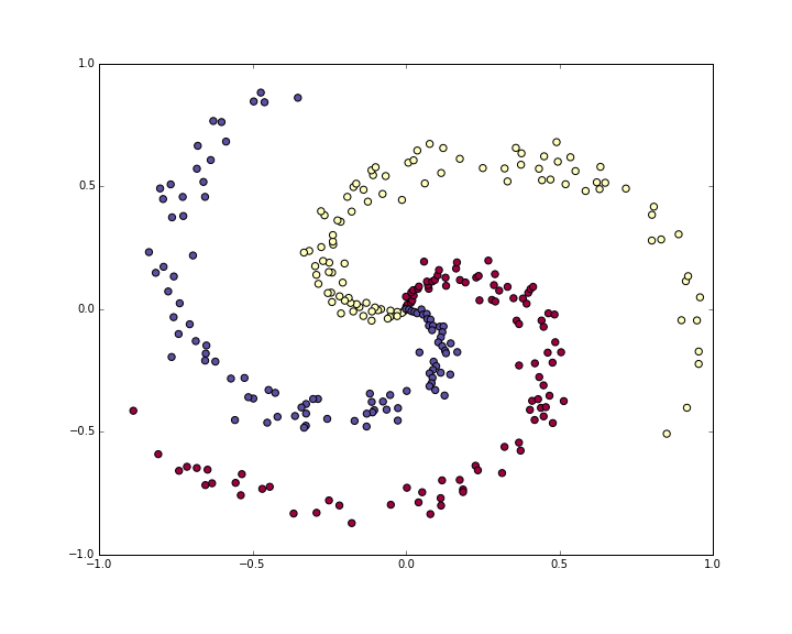The toy spiral data consists of three classes (blue, red, yellow) that are not linearly separable.

장난감 나선형 데이터는 선형으로 나뉘지 않는 세 클래스(파랑, 빨강, 노랑)로 이루어져 있다.

역주. 코드 다섯 줄이 어떻게 나선이 되는지 짚어두면 그림이 훨씬 잘 읽힌다. 클래스 하나마다 반지름 r은 0에서 1까지 고르게 늘어나고, 각도 t는 j*4에서 (j+1)*4까지, 곧 4라디안(약 229도)을 쓸고 지나간다. 점을 (r*sin(t), r*cos(t))로 놓으면 원점에서 멀어지는 동시에 계속 돌아가므로 팔 하나가 그려진다. 클래스 j마다 시작 각도를 4라디안씩 어긋나게 잡았으니 팔 세 개가 원 둘레에 대략 고르게 벌어지고, np.random.randn(N)*0.2는 각도에 잡음을 얹어 팔 가장자리를 흐트러뜨린다.

선형으로 나뉘지 않는 이유도 여기서 보인다. 원점 근처에서는 r이 작아 세 클래스의 점들이 한자리에 모여 뒤섞이고, 팔은 저마다 229도를 돌아가므로 어떤 직선을 그어도 한 클래스를 나머지 둘에서 떼어낼 수 없다. 선형 분류기가 그릴 수 있는 결정 경계는 직선뿐이니, 뒤에서 정확도가 49%에서 멈추는 것은 데이터를 만드는 이 다섯 줄에서 이미 정해진 셈이다.

Normally we would want to preprocess the dataset so that each feature has zero mean and unit standard deviation, but in this case the features are already in a nice range from -1 to 1, so we skip this step.

보통은 각 특징의 평균이 0이고 표준편차가 1이 되도록 데이터셋을 전처리하고 싶겠지만, 지금은 특징이 이미 -1에서 1 사이의 좋은 범위에 들어 있으므로 이 단계는 건너뛴다.

Training a Softmax Linear Classifier

Initialize the parameters

Lets first train a Softmax classifier on this classification dataset. As we saw in the previous sections, the Softmax classifier has a linear score function and uses the cross-entropy loss. The parameters of the linear classifier consist of a weight matrix W and a bias vector b for each class. Lets first initialize these parameters to be random numbers:

먼저 이 분류 데이터셋에 Softmax 분류기를 학습시켜보자. 앞의 절들에서 봤듯 Softmax 분류기는 선형 점수 함수를 쓰고 교차 엔트로피 손실을 쓴다. 선형 분류기의 매개변수는 가중치 행렬 W와 클래스마다 하나씩 있는 편향 벡터 b로 이루어진다. 우선 이 매개변수들을 난수로 초기화한다.

# initialize parameters randomly
W = 0.01 * np.random.randn(D,K)
b = np.zeros((1,K))

Recall that we D = 2 is the dimensionality and K = 3 is the number of classes.

D = 2가 차원 수이고 K = 3이 클래스 개수라는 것을 떠올리자.

Compute the class scores

Since this is a linear classifier, we can compute all class scores very simply in parallel with a single matrix multiplication:

선형 분류기이므로 모든 클래스 점수를 행렬 곱 한 번으로 아주 간단히 한꺼번에 계산할 수 있다.

# compute class scores for a linear classifier
scores = np.dot(X, W) + b

In this example we have 300 2-D points, so after this multiplication the array scores will have size [300 x 3], where each row gives the class scores corresponding to the 3 classes (blue, red, yellow).

이 예제에는 2차원 점이 300개 있으므로 이 곱셈을 마치고 나면 배열 scores의 크기는 [300 x 3]이 되고, 각 행은 세 클래스(파랑, 빨강, 노랑)에 대응하는 클래스 점수를 담는다.

Compute the loss

The second key ingredient we need is a loss function, which is a differentiable objective that quantifies our unhappiness with the computed class scores. Intuitively, we want the correct class to have a higher score than the other classes. When this is the case, the loss should be low and otherwise the loss should be high. There are many ways to quantify this intuition, but in this example lets use the cross-entropy loss that is associated with the Softmax classifier. Recall that if \(f\) is the array of class scores for a single example (e.g. array of 3 numbers here), then the Softmax classifier computes the loss for that example as:

\[L_i = -\log\left(\frac{e^{f_{y_i}}}{ \sum_j e^{f_j} }\right)\]

두 번째로 필요한 핵심 재료는 손실 함수다. 손실 함수는 계산된 클래스 점수가 얼마나 마음에 들지 않는지를 수치로 나타내는 미분 가능한 목적 함수다. 직관적으로 우리는 정답 클래스의 점수가 다른 클래스들보다 높기를 바란다. 그럴 때는 손실이 낮아야 하고 그렇지 않으면 손실이 높아야 한다. 이 직관을 수치로 옮기는 방법은 여럿 있지만, 이 예제에서는 Softmax 분류기와 짝을 이루는 교차 엔트로피 손실을 쓴다. \(f\)가 예제 하나에 대한 클래스 점수 배열(여기서는 숫자 세 개짜리 배열)이라면 Softmax 분류기가 그 예제의 손실을 다음과 같이 계산한다는 것을 떠올리자.

We can see that the Softmax classifier interprets every element of \(f\) as holding the (unnormalized) log probabilities of the three classes. We exponentiate these to get (unnormalized) probabilities, and then normalize them to get probabilites. Therefore, the expression inside the log is the normalized probability of the correct class. Note how this expression works: this quantity is always between 0 and 1. When the probability of the correct class is very small (near 0), the loss will go towards (positive) infinity. Conversely, when the correct class probability goes towards 1, the loss will go towards zero because \(log(1) = 0\). Hence, the expression for \(L_i\) is low when the correct class probability is high, and it’s very high when it is low.

여기서 Softmax 분류기가 \(f\)의 각 원소를 세 클래스의 정규화되지 않은 로그 확률로 해석한다는 것을 알 수 있다. 이 값들에 지수를 취해 (정규화되지 않은) 확률을 얻고, 그것을 정규화(normalization)해 확률을 얻는다. 그러므로 로그 안의 식은 정답 클래스의 정규화된 확률이다. 이 식이 어떻게 동작하는지 보자. 이 값은 언제나 0과 1 사이다. 정답 클래스의 확률이 아주 작으면(0에 가까우면) 손실은 (양의) 무한대로 간다. 반대로 정답 클래스 확률이 1로 다가가면 \(log(1) = 0\)이므로 손실은 0으로 간다. 따라서 \(L_i\) 식은 정답 클래스 확률이 높을 때 낮고, 낮을 때 아주 높다.

Recall also that the full Softmax classifier loss is then defined as the average cross-entropy loss over the training examples and the regularization:

\[L = \underbrace{ \frac{1}{N} \sum_i L_i }_\text{data loss} + \underbrace{ \frac{1}{2} \lambda \sum_k\sum_l W_{k,l}^2 }_\text{regularization loss} \\\\\]

그리고 Softmax 분류기의 전체 손실이 학습 예제들에 대한 교차 엔트로피 손실의 평균과 정규화(regularization) 항으로 정의된다는 것도 떠올리자.

Given the array of scores we’ve computed above, we can compute the loss. First, the way to obtain the probabilities is straight forward:

위에서 계산한 scores 배열이 있으면 손실을 계산할 수 있다. 먼저 확률을 얻는 방법은 간단하다.

num_examples = X.shape[0]
# get unnormalized probabilities
exp_scores = np.exp(scores)
# normalize them for each example
probs = exp_scores / np.sum(exp_scores, axis=1, keepdims=True)

We now have an array probs of size [300 x 3], where each row now contains the class probabilities. In particular, since we’ve normalized them every row now sums to one. We can now query for the log probabilities assigned to the correct classes in each example:

이제 크기가 [300 x 3]인 배열 probs가 생겼고 각 행은 클래스 확률을 담는다. 특히 정규화를 했으므로 이제 모든 행의 합이 1이다. 이제 각 예제에서 정답 클래스에 매겨진 로그 확률을 뽑아낼 수 있다.

correct_logprobs = -np.log(probs[range(num_examples),y])

The array correct_logprobs is a 1D array of just the probabilities assigned to the correct classes for each example. The full loss is then the average of these log probabilities and the regularization loss:

배열 correct_logprobs는 예제마다 정답 클래스에 매겨진 확률만 모아둔 1차원 배열이다. 전체 손실은 이 로그 확률들의 평균에 정규화 손실을 더한 것이다.

# compute the loss: average cross-entropy loss and regularization
data_loss = np.sum(correct_logprobs)/num_examples
reg_loss = 0.5*reg*np.sum(W*W)
loss = data_loss + reg_loss

In this code, the regularization strength \(\lambda\) is stored inside the reg. The convenience factor of 0.5 multiplying the regularization will become clear in a second. Evaluating this in the beginning (with random parameters) might give us loss = 1.1, which is -np.log(1.0/3), since with small initial random weights all probabilities assigned to all classes are about one third. We now want to make the loss as low as possible, with loss = 0 as the absolute lower bound. But the lower the loss is, the higher are the probabilities assigned to the correct classes for all examples.

이 코드에서 정규화 세기 \(\lambda\)는 reg에 들어 있다. 정규화 항에 곱한 0.5라는 편의상의 인자가 왜 붙었는지는 잠시 뒤에 분명해진다. 처음에 (무작위 매개변수로) 이 값을 계산해보면 loss = 1.1쯤이 나오는데, 이것은 -np.log(1.0/3)이다. 초기 가중치가 작은 난수이면 모든 클래스에 매겨지는 확률이 전부 3분의 1 언저리이기 때문이다. 이제 우리는 손실을 가능한 한 낮추려 하며, 절대적인 하한은 loss = 0이다. 그리고 손실이 낮을수록 모든 예제에서 정답 클래스에 매겨진 확률이 높다는 뜻이다.

Computing the Analytic Gradient with Backpropagation

We have a way of evaluating the loss, and now we have to minimize it. We’ll do so with gradient descent. That is, we start with random parameters (as shown above), and evaluate the gradient of the loss function with respect to the parameters, so that we know how we should change the parameters to decrease the loss. Lets introduce the intermediate variable \(p\), which is a vector of the (normalized) probabilities. The loss for one example is:

\[p_k = \frac{e^{f_k}}{ \sum_j e^{f_j} } \hspace{1in} L_i =-\log\left(p_{y_i}\right)\]

손실을 계산하는 방법은 마련했으니 이제 그것을 최소화해야 한다. 경사 하강법으로 한다. 즉 위에서처럼 무작위 매개변수에서 출발해, 매개변수에 대한 손실 함수의 기울기를 계산하고, 그것을 보고 손실을 줄이려면 매개변수를 어떻게 바꿔야 하는지 알아낸다. 중간 변수 \(p\)를 도입하자. \(p\)는 (정규화된) 확률들의 벡터다. 예제 하나의 손실은 다음과 같다.

We now wish to understand how the computed scores inside \(f\) should change to decrease the loss \(L_i\) that this example contributes to the full objective. In other words, we want to derive the gradient \(\partial L_i / \partial f_k\). The loss \(L_i\) is computed from \(p\), which in turn depends on \(f\). It’s a fun exercise to the reader to use the chain rule to derive the gradient, but it turns out to be extremely simple and interpretible in the end, after a lot of things cancel out:

\[\frac{\partial L_i }{ \partial f_k } = p_k - \mathbb{1}(y_i = k)\]

이제 이 예제가 전체 목적 함수에 보태는 손실 \(L_i\)를 줄이려면 \(f\) 안에 계산된 점수들이 어떻게 바뀌어야 하는지 알고 싶다. 다시 말해 기울기 \(\partial L_i / \partial f_k\)를 유도하려는 것이다. 손실 \(L_i\)는 \(p\)로부터 계산되고 \(p\)는 다시 \(f\)에 의존한다. 연쇄 법칙으로 이 기울기를 유도해보는 것은 독자에게 남겨두는 재미있는 연습이지만, 여러 항이 서로 지워지고 나면 결국 극도로 간단하고 해석하기 좋은 식이 남는다.

역주. 원문이 남겨둔 연습을 두 줄만 해보면 왜 이렇게까지 간단해지는지 보인다. \(L_i = -\log p_{y_i}\)이므로 연쇄 법칙의 첫 마디는 다음과 같다.

\[\frac{\partial L_i}{\partial f_k} = -\frac{1}{p_{y_i}} \frac{\partial p_{y_i}}{\partial f_k}\]

남은 것은 softmax를 미분하는 일뿐인데, 이것은 미분하는 자리 \(k\)가 정답 자리인지 아닌지에 따라 갈린다. \(p_{y_i} = e^{f_{y_i}} / \sum_j e^{f_j}\)에 몫의 미분을 그대로 적용하면 \(k = y_i\)일 때는 분자도 함께 미분되어 \(p_{y_i}(1 - p_{y_i})\)가 나오고, \(k \neq y_i\)일 때는 분모만 미분되어 \(-p_{y_i} p_k\)가 나온다. 지시 함수를 쓰면 두 경우가 한 식으로 묶인다.

\[\frac{\partial p_{y_i}}{\partial f_k} = p_{y_i}\left(\mathbb{1}(y_i = k) - p_k\right)\]

이것을 앞의 식에 넣으면 \(p_{y_i}\)가 통째로 약분되어 사라지고 부호가 뒤집혀 \(p_k - \mathbb{1}(y_i = k)\)만 남는다. 원문이 “여러 항이 서로 지워진다”고 한 것이 이 약분이며, 확률 벡터에서 정답 자리 하나만 1을 빼면 된다는 결론이 여기서 나온다.

Notice how elegant and simple this expression is. Suppose the probabilities we computed were p = [0.2, 0.3, 0.5], and that the correct class was the middle one (with probability 0.3). According to this derivation the gradient on the scores would be df = [0.2, -0.7, 0.5]. Recalling what the interpretation of the gradient, we see that this result is highly intuitive: increasing the first or last element of the score vector f (the scores of the incorrect classes) leads to an increased loss (due to the positive signs +0.2 and +0.5) - and increasing the loss is bad, as expected. However, increasing the score of the correct class has negative influence on the loss. The gradient of -0.7 is telling us that increasing the correct class score would lead to a decrease of the loss \(L_i\), which makes sense.

이 식이 얼마나 우아하고 간단한지 보자. 계산된 확률이 p = [0.2, 0.3, 0.5]이고 정답 클래스가 가운데 것(확률 0.3)이었다고 하자. 이 유도에 따르면 점수에 대한 기울기는 df = [0.2, -0.7, 0.5]가 된다. 기울기를 어떻게 해석하는지 떠올려보면 이 결과가 대단히 직관적이라는 것을 알 수 있다. 점수 벡터 f의 첫 번째나 마지막 원소(오답 클래스의 점수)를 키우면 손실이 늘어난다(+0.2와 +0.5라는 양의 부호 때문이다). 그리고 손실이 늘어나는 것은 예상대로 나쁜 일이다. 반면 정답 클래스의 점수를 키우면 손실에 음의 영향을 준다. -0.7이라는 기울기는 정답 클래스 점수를 키우면 손실 \(L_i\)가 줄어든다고 말해주고 있고, 이는 말이 된다.

All of this boils down to the following code. Recall that probs stores the probabilities of all classes (as rows) for each example. To get the gradient on the scores, which we call dscores, we proceed as follows:

이 모든 것이 다음 코드로 압축된다. probs가 예제마다 모든 클래스의 확률을 (행으로) 담고 있다는 것을 떠올리자. 점수에 대한 기울기, 곧 dscores를 구하려면 다음과 같이 하면 된다.

dscores = probs
dscores[range(num_examples),y] -= 1
dscores /= num_examples

역주. dscores = probs는 배열을 복사하지 않는다. 두 이름이 같은 배열을 가리키므로 이어지는 -= 1과 /= num_examples는 probs를 제자리에서 고쳐 쓴다. 아래 학습 루프에서는 반복마다 probs를 새로 계산하니 아무 문제가 없지만, 대화형으로 한 줄씩 따라 하다가 나중에 probs를 다시 들여다보면 행의 합이 1이 아니어서 당황하게 된다.

실제로 이 세 줄을 지나고 나면 각 행의 합은 0이 된다. probs 한 행의 합이 1이었는데 정답 자리 하나에서만 1을 뺐으니 합이 0이 되고, 0을 num_examples로 나눠도 0이기 때문이다. 이 “행마다 합이 0”은 그 자체로 뜻이 있다. 한 예제의 점수 전체를 같은 값만큼 밀어 올려도 softmax 확률은 변하지 않으므로 그 방향으로는 손실이 움직이지 않아야 하고, 따라서 그 방향의 기울기도 0이어야 한다.

Lastly, we had that scores = np.dot(X, W) + b, so armed with the gradient on scores (stored in dscores), we can now backpropagate into W and b:

마지막으로 scores = np.dot(X, W) + b였으므로, scores에 대한 기울기(dscores에 들어 있다)를 손에 넣은 이상 이제 W와 b로 역전파할 수 있다.

dW = np.dot(X.T, dscores)
db = np.sum(dscores, axis=0, keepdims=True)
dW += reg*W # don't forget the regularization gradient

Where we see that we have backpropped through the matrix multiply operation, and also added the contribution from the regularization. Note that the regularization gradient has the very simple form reg*W since we used the constant 0.5 for its loss contribution (i.e. \(\frac{d}{dw} ( \frac{1}{2} \lambda w^2) = \lambda w\). This is a common convenience trick that simplifies the gradient expression.

여기서 우리가 행렬 곱 연산을 통과해 역전파했고 정규화가 보태는 몫도 더했다는 것을 볼 수 있다. 정규화 기울기가 reg*W라는 아주 간단한 형태인 것은 손실에 보태는 몫에 상수 0.5를 곱해뒀기 때문이다(즉 \(\frac{d}{dw} ( \frac{1}{2} \lambda w^2) = \lambda w\)). 기울기 식을 간단하게 만드는, 흔히 쓰는 편의상의 요령이다.

Performing a parameter update

Now that we’ve evaluated the gradient we know how every parameter influences the loss function. We will now perform a parameter update in the negative gradient direction to decrease the loss:

기울기를 계산했으니 이제 모든 매개변수가 손실 함수에 어떻게 영향을 주는지 안다. 이제 손실을 줄이기 위해 기울기의 반대 방향으로 매개변수를 갱신한다.

# perform a parameter update
W += -step_size * dW
b += -step_size * db

Putting it all together: Training a Softmax Classifier

Putting all of this together, here is the full code for training a Softmax classifier with Gradient descent:

이 모든 것을 합치면, 경사 하강법으로 Softmax 분류기를 학습시키는 전체 코드는 다음과 같다.

#Train a Linear Classifier

# initialize parameters randomly
W = 0.01 * np.random.randn(D,K)
b = np.zeros((1,K))

# some hyperparameters
step_size = 1e-0
reg = 1e-3 # regularization strength

# gradient descent loop
num_examples = X.shape[0]
for i in range(200):

  # evaluate class scores, [N x K]
  scores = np.dot(X, W) + b

  # compute the class probabilities
  exp_scores = np.exp(scores)
  probs = exp_scores / np.sum(exp_scores, axis=1, keepdims=True) # [N x K]

  # compute the loss: average cross-entropy loss and regularization
  correct_logprobs = -np.log(probs[range(num_examples),y])
  data_loss = np.sum(correct_logprobs)/num_examples
  reg_loss = 0.5*reg*np.sum(W*W)
  loss = data_loss + reg_loss
  if i % 10 == 0:
    print "iteration %d: loss %f" % (i, loss)

  # compute the gradient on scores
  dscores = probs
  dscores[range(num_examples),y] -= 1
  dscores /= num_examples

  # backpropate the gradient to the parameters (W,b)
  dW = np.dot(X.T, dscores)
  db = np.sum(dscores, axis=0, keepdims=True)

  dW += reg*W # regularization gradient

  # perform a parameter update
  W += -step_size * dW
  b += -step_size * db

Running this prints the output:

이것을 실행하면 다음이 출력된다.

iteration 0: loss 1.096956
iteration 10: loss 0.917265
iteration 20: loss 0.851503
iteration 30: loss 0.822336
iteration 40: loss 0.807586
iteration 50: loss 0.799448
iteration 60: loss 0.794681
iteration 70: loss 0.791764
iteration 80: loss 0.789920
iteration 90: loss 0.788726
iteration 100: loss 0.787938
iteration 110: loss 0.787409
iteration 120: loss 0.787049
iteration 130: loss 0.786803
iteration 140: loss 0.786633
iteration 150: loss 0.786514
iteration 160: loss 0.786431
iteration 170: loss 0.786373
iteration 180: loss 0.786331
iteration 190: loss 0.786302

We see that we’ve converged to something after about 190 iterations. We can evaluate the training set accuracy:

190번쯤 반복하고 나면 어딘가로 수렴한 것을 볼 수 있다. 학습 집합 정확도를 계산해보자.

# evaluate training set accuracy
scores = np.dot(X, W) + b
predicted_class = np.argmax(scores, axis=1)
print 'training accuracy: %.2f' % (np.mean(predicted_class == y))

This prints 49%. Not very good at all, but also not surprising given that the dataset is constructed so it is not linearly separable. We can also plot the learned decision boundaries:

49%가 출력된다. 전혀 좋지 않지만, 데이터셋 자체가 선형으로 나뉘지 않도록 만들어졌다는 것을 생각하면 놀랄 일도 아니다. 학습된 결정 경계를 그려볼 수도 있다.

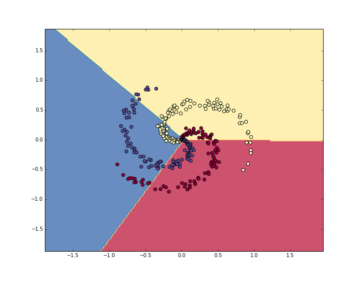Linear classifier fails to learn the toy spiral dataset.

선형 분류기는 장난감 나선형 데이터셋을 학습하는 데 실패한다.

Training a Neural Network

Clearly, a linear classifier is inadequate for this dataset and we would like to use a Neural Network. One additional hidden layer will suffice for this toy data. We will now need two sets of weights and biases (for the first and second layers):

이 데이터셋에는 선형 분류기가 분명히 모자라니 신경망을 쓰고 싶어진다. 이 장난감 데이터에는 은닉층 하나만 더 있으면 충분하다. 이제 가중치와 편향이 (첫 번째 층과 두 번째 층에 하나씩) 두 벌 필요하다.

# initialize parameters randomly
h = 100 # size of hidden layer
W = 0.01 * np.random.randn(D,h)
b = np.zeros((1,h))
W2 = 0.01 * np.random.randn(h,K)
b2 = np.zeros((1,K))

The forward pass to compute scores now changes form:

점수를 계산하는 순전파는 이제 모양이 달라진다.

# evaluate class scores with a 2-layer Neural Network
hidden_layer = np.maximum(0, np.dot(X, W) + b) # note, ReLU activation
scores = np.dot(hidden_layer, W2) + b2

Notice that the only change from before is one extra line of code, where we first compute the hidden layer representation and then the scores based on this hidden layer. Crucially, we’ve also added a non-linearity, which in this case is simple ReLU that thresholds the activations on the hidden layer at zero.

앞과 달라진 곳은 코드 한 줄이 늘어난 것뿐이라는 데 주목하자. 먼저 은닉층 표현을 계산하고, 그다음에 이 은닉층을 바탕으로 점수를 계산한다. 결정적으로, 비선형성도 함께 넣었다. 여기서는 은닉층의 활성값을 0에서 잘라내는 간단한 ReLU다.

Everything else remains the same. We compute the loss based on the scores exactly as before, and get the gradient for the scores dscores exactly as before. However, the way we backpropagate that gradient into the model parameters now changes form, of course. First lets backpropagate the second layer of the Neural Network. This looks identical to the code we had for the Softmax classifier, except we’re replacing X (the raw data), with the variable hidden_layer):

나머지는 전부 그대로다. 점수를 바탕으로 손실을 계산하는 것도 앞과 똑같고, 점수에 대한 기울기 dscores를 구하는 것도 앞과 똑같다. 다만 그 기울기를 모델 매개변수로 역전파하는 방식은 당연히 모양이 달라진다. 먼저 신경망의 두 번째 층을 역전파해보자. Softmax 분류기에서 썼던 코드와 똑같아 보이는데, X(원시 데이터) 자리에 변수 hidden_layer가 들어간 것만 다르다.

# backpropate the gradient to the parameters
# first backprop into parameters W2 and b2
dW2 = np.dot(hidden_layer.T, dscores)
db2 = np.sum(dscores, axis=0, keepdims=True)

However, unlike before we are not yet done, because hidden_layer is itself a function of other parameters and the data! We need to continue backpropagation through this variable. Its gradient can be computed as:

그런데 앞과 달리 아직 끝난 것이 아니다. hidden_layer 자체가 다른 매개변수들과 데이터의 함수이기 때문이다. 이 변수를 지나 역전파를 계속해야 한다. 그 기울기는 다음과 같이 계산할 수 있다.

dhidden = np.dot(dscores, W2.T)

Now we have the gradient on the outputs of the hidden layer. Next, we have to backpropagate the ReLU non-linearity. This turns out to be easy because ReLU during the backward pass is effectively a switch. Since \(r = max(0, x)\), we have that \(\frac{dr}{dx} = 1(x > 0)\). Combined with the chain rule, we see that the ReLU unit lets the gradient pass through unchanged if its input was greater than 0, but kills it if its input was less than zero during the forward pass. Hence, we can backpropagate the ReLU in place simply with:

이제 은닉층 출력에 대한 기울기를 얻었다. 다음으로 ReLU 비선형성을 역전파해야 한다. 이것은 쉬운 일인데, 역방향 진행에서 ReLU가 사실상 스위치이기 때문이다. \(r = max(0, x)\)이므로 \(\frac{dr}{dx} = 1(x > 0)\)이다. 여기에 연쇄 법칙을 합쳐 보면, ReLU 유닛은 순전파 때 입력이 0보다 컸으면 기울기를 그대로 통과시키고 입력이 0보다 작았으면 죽여버린다는 것을 알 수 있다. 따라서 ReLU의 역전파는 다음과 같이 제자리에서 간단히 해낼 수 있다.

# backprop the ReLU non-linearity
dhidden[hidden_layer <= 0] = 0

역주. 마스크의 조건이 순전파의 입력 np.dot(X, W) + b가 아니라 출력 hidden_layer인 것에 잠깐 걸릴 수 있는데, 둘은 같은 조건이다. hidden_layer = max(0, x)이므로 hidden_layer <= 0인 자리는 정확히 x <= 0인 자리이고, 그래서 순전파의 입력을 따로 들고 있지 않아도 된다. 활성값을 저장해두는 것만으로 역방향 진행이 되므로 메모리도 아낀다.

경계인 \(x = 0\)은 ReLU가 미분 불가능한 꺾임이지만, 이 코드는 그 자리를 기울기가 0인 쪽으로 넘긴다. 부동소수점에서 값이 정확히 0이 되는 일은 거의 없고 어느 쪽으로 정하든 학습에 차이가 없어, 관례상 한쪽으로 정해두고 넘어간다.

And now we finally continue to the first layer weights and biases:

그리고 이제 마침내 첫 번째 층의 가중치와 편향까지 이어간다.

# finally into W,b
dW = np.dot(X.T, dhidden)
db = np.sum(dhidden, axis=0, keepdims=True)

We’re done! We have the gradients dW,db,dW2,db2 and can perform the parameter update. Everything else remains unchanged. The full code looks very similar:

끝났다! 기울기 dW,db,dW2,db2를 모두 얻었으니 매개변수를 갱신할 수 있다. 나머지는 하나도 바뀌지 않는다. 전체 코드는 앞의 것과 매우 비슷하다.

# initialize parameters randomly
h = 100 # size of hidden layer
W = 0.01 * np.random.randn(D,h)
b = np.zeros((1,h))
W2 = 0.01 * np.random.randn(h,K)
b2 = np.zeros((1,K))

# some hyperparameters
step_size = 1e-0
reg = 1e-3 # regularization strength

# gradient descent loop
num_examples = X.shape[0]
for i in range(10000):

  # evaluate class scores, [N x K]
  hidden_layer = np.maximum(0, np.dot(X, W) + b) # note, ReLU activation
  scores = np.dot(hidden_layer, W2) + b2

  # compute the class probabilities
  exp_scores = np.exp(scores)
  probs = exp_scores / np.sum(exp_scores, axis=1, keepdims=True) # [N x K]

  # compute the loss: average cross-entropy loss and regularization
  correct_logprobs = -np.log(probs[range(num_examples),y])
  data_loss = np.sum(correct_logprobs)/num_examples
  reg_loss = 0.5*reg*np.sum(W*W) + 0.5*reg*np.sum(W2*W2)
  loss = data_loss + reg_loss
  if i % 1000 == 0:
    print "iteration %d: loss %f" % (i, loss)

  # compute the gradient on scores
  dscores = probs
  dscores[range(num_examples),y] -= 1
  dscores /= num_examples

  # backpropate the gradient to the parameters
  # first backprop into parameters W2 and b2
  dW2 = np.dot(hidden_layer.T, dscores)
  db2 = np.sum(dscores, axis=0, keepdims=True)
  # next backprop into hidden layer
  dhidden = np.dot(dscores, W2.T)
  # backprop the ReLU non-linearity
  dhidden[hidden_layer <= 0] = 0
  # finally into W,b
  dW = np.dot(X.T, dhidden)
  db = np.sum(dhidden, axis=0, keepdims=True)

  # add regularization gradient contribution
  dW2 += reg * W2
  dW += reg * W

  # perform a parameter update
  W += -step_size * dW
  b += -step_size * db
  W2 += -step_size * dW2
  b2 += -step_size * db2

This prints:

다음이 출력된다.

iteration 0: loss 1.098744
iteration 1000: loss 0.294946
iteration 2000: loss 0.259301
iteration 3000: loss 0.248310
iteration 4000: loss 0.246170
iteration 5000: loss 0.245649
iteration 6000: loss 0.245491
iteration 7000: loss 0.245400
iteration 8000: loss 0.245335
iteration 9000: loss 0.245292

The training accuracy is now:

학습 정확도는 이제 다음과 같다.

# evaluate training set accuracy
hidden_layer = np.maximum(0, np.dot(X, W) + b)
scores = np.dot(hidden_layer, W2) + b2
predicted_class = np.argmax(scores, axis=1)
print 'training accuracy: %.2f' % (np.mean(predicted_class == y))

Which prints 98%!. We can also visualize the decision boundaries:

98%가 출력된다! 결정 경계를 시각화해볼 수도 있다.

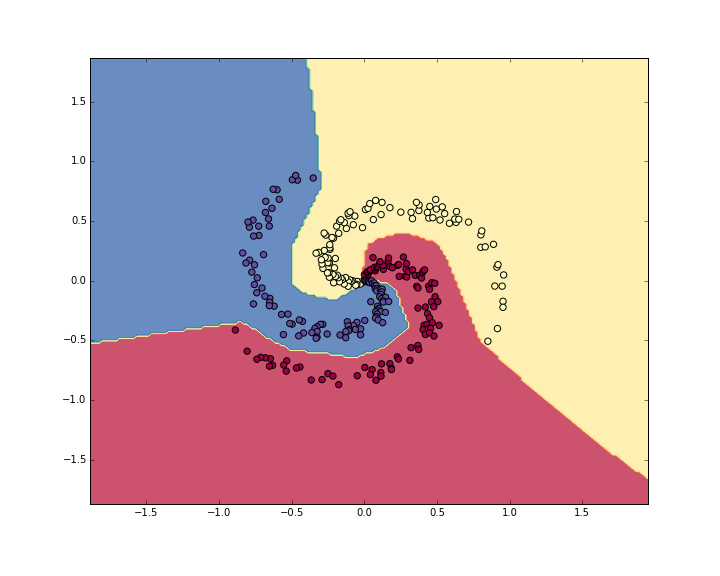Neural Network classifier crushes the spiral dataset.

신경망 분류기는 나선형 데이터셋을 가볍게 제압한다.

보충: 비선형성을 빼면 은닉층을 더해도 왜 소용이 없는지 재어보기

원문은 은닉층을 더한 것 못지않게 “결정적으로, 비선형성도 함께 넣었다”고 짚지만, 왜 그것이 결정적인지는 보여주지 않고 넘어간다. 재어보면 된다. 바로 위 2층 코드에서 np.maximum(0, ...) 하나만 빼고 나머지 — 은닉 유닛 100개, 학습률, 정규화 세기, 반복 횟수, 심지어 초깃값까지 — 를 그대로 두면 무슨 일이 일어나는지 보자. 원문 코드는 Python 2 문법(print "..." % (...))이라 Python 3에서는 그대로 돌지 않으므로 출력하는 부분만 고쳤고, 결과가 실행할 때마다 흔들리지 않도록 난수를 고정했다.

import numpy as np

np.random.seed(0)

N, D, K, h = 100, 2, 3, 100
X = np.zeros((N*K, D))
y = np.zeros(N*K, dtype='uint8')
for j in range(K):
    ix = range(N*j, N*(j+1))
    r = np.linspace(0.0, 1, N)
    t = np.linspace(j*4, (j+1)*4, N) + np.random.randn(N)*0.2
    X[ix] = np.c_[r*np.sin(t), r*np.cos(t)]
    y[ix] = j

step_size, reg, num_examples = 1e-0, 1e-3, X.shape[0]

def train(relu):
    np.random.seed(1)  # 두 신경망이 똑같은 초깃값에서 출발하게 한다
    W, b = 0.01 * np.random.randn(D, h), np.zeros((1, h))
    W2, b2 = 0.01 * np.random.randn(h, K), np.zeros((1, K))
    for i in range(10000):
        z = np.dot(X, W) + b
        hidden_layer = np.maximum(0, z) if relu else z   # 갈리는 곳은 이 한 줄뿐이다
        scores = np.dot(hidden_layer, W2) + b2
        exp_scores = np.exp(scores)
        probs = exp_scores / np.sum(exp_scores, axis=1, keepdims=True)
        dscores = probs
        dscores[range(num_examples), y] -= 1
        dscores /= num_examples
        dW2 = np.dot(hidden_layer.T, dscores)
        db2 = np.sum(dscores, axis=0, keepdims=True)
        dhidden = np.dot(dscores, W2.T)
        if relu:
            dhidden[hidden_layer <= 0] = 0
        dW = np.dot(X.T, dhidden)
        db = np.sum(dhidden, axis=0, keepdims=True)
        dW2 += reg * W2
        dW += reg * W
        W += -step_size * dW
        b += -step_size * db
        W2 += -step_size * dW2
        b2 += -step_size * db2
    z = np.dot(X, W) + b
    hidden_layer = np.maximum(0, z) if relu else z
    scores = np.dot(hidden_layer, W2) + b2
    return np.mean(np.argmax(scores, axis=1) == y), (W, b, W2, b2)

acc_relu, _ = train(relu=True)
acc_lin, (W, b, W2, b2) = train(relu=False)
print('ReLU 있음: 학습 정확도 %.2f' % acc_relu)
print('ReLU 없음: 학습 정확도 %.2f' % acc_lin)

# ReLU 없는 2층 신경망은 층을 접어 W 한 벌로 만들 수 있다
W_eff, b_eff = np.dot(W, W2), np.dot(b, W2) + b2
print('접어낸 W_eff의 모양:', W_eff.shape, '(선형 분류기의 W와 같다)')
two_layer = np.dot(np.dot(X, W) + b, W2) + b2
folded = np.dot(X, W_eff) + b_eff
print('두 층으로 낸 점수와 접어서 낸 점수의 최대 차이: %.2e' % np.abs(two_layer - folded).max())

ReLU 있음: 학습 정확도 0.98
ReLU 없음: 학습 정확도 0.49
접어낸 W_eff의 모양: (2, 3) (선형 분류기의 W와 같다)
두 층으로 낸 점수와 접어서 낸 점수의 최대 차이: 1.78e-15

ReLU를 뺀 신경망은 매개변수를 603개나 가지고 10000번을 학습했는데도 정확도가 0.49에서 멈춘다. 원문의 선형 분류기가 매개변수 아홉 개로 200번 만에 도달한 바로 그 숫자다. 이유는 마지막 두 줄이 보여준다. 비선형성이 없으면 두 층은 그저 행렬 곱을 두 번 하는 것이고, 행렬 곱 두 번은 행렬 곱 한 번으로 접힌다. W.dot(W2)로 층을 접으면 크기가 [2 x 3]인 행렬 하나가 나오는데 이것은 선형 분류기의 W와 정확히 같은 모양이며, 접어서 낸 점수는 두 층으로 낸 점수와 1e-15 수준, 곧 부동소수점 오차만큼만 다르다. 은닉 유닛을 100개가 아니라 10000개로 늘려도 달라지지 않는다. 중간 행렬이 아무리 커도 곱하고 나면 [2 x 3]으로 되돌아가기 때문이다.

층을 쌓아 얻는 것은 층 그 자체가 아니라 층 사이에 낀 비선형성이다. 원문이 한 줄 늘어난 것을 두고 “결정적으로”라고 쓴 이유가 이것이다.

Summary

We’ve worked with a toy 2D dataset and trained both a linear network and a 2-layer Neural Network. We saw that the change from a linear classifier to a Neural Network involves very few changes in the code. The score function changes its form (1 line of code difference), and the backpropagation changes its form (we have to perform one more round of backprop through the hidden layer to the first layer of the network).

장난감 2차원 데이터셋을 가지고 선형 신경망과 2층 신경망을 모두 학습시켜봤다. 선형 분류기에서 신경망으로 넘어가는 데 코드가 거의 달라지지 않는다는 것을 봤다. 점수 함수의 모양이 바뀌고(코드 한 줄 차이), 역전파의 모양이 바뀐다(은닉층을 지나 신경망의 첫 번째 층까지 역전파를 한 번 더 해야 한다).

• You may want to look at this IPython Notebook code rendered as HTML.
• Or download the ipynb file

• 이 코드를 IPython Notebook으로 HTML로 렌더링해둔 것을 봐도 좋다.
• 아니면 ipynb 파일을 내려받아도 된다.