12. Recurrent Neural Networks

원문: Recurrent Neural Networks — CS231n: Convolutional Neural Networks for Visual Recognition (Stanford University) · © 2015 Andrej Karpathy, MIT License

원문을 문단 단위로 인용하고 그 아래에 한국어 번역을 붙였다. 인용 블록이 원문, 그 아래 문단이 번역이며, 역주 박스와 보충 섹션은 원문에 없는 추가 내용이다.

Table of Contents:

목차는 다음과 같다.

• Introduction to RNN
• RNN example as Character-level language model
• Multilayer RNNs
• Long-Short Term Memory (LSTM)

• RNN 소개
• 문자 단위 언어 모델 예시로 보는 RNN
• 다층 RNN
• Long-Short Term Memory (LSTM)

Introduction to RNN

In this lecture note, we’re going to be talking about the Recurrent Neural Networks (RNNs). One great thing about the RNNs is that they offer a lot of flexibility on how we wire up the neural network architecture. Normally when we’re working with neural networks (Figure 1), we are given a fixed sized input vector (red), then we process it with some hidden layers (green), and we produce a fixed sized output vector (blue) as depicted in the leftmost model (“Vanilla” Neural Networks) in Figure 1. While “Vanilla” Neural Networks receive a single input and produce one label for that image, there are tasks where the model produce a sequence of outputs as shown in the one-to-many model in Figure 1. Recurrent Neural Networks allow us to operate over sequences of input, output, or both at the same time.

이 강의 노트에서는 순환 신경망(Recurrent Neural Networks)을 다룬다. RNN의 큰 장점 하나는 신경망 구조를 어떻게 연결할지에 있어 상당한 유연성을 준다는 점이다. 신경망을 다룰 때(Figure 1) 보통은 고정된 크기의 입력 벡터(빨간색)를 받아 몇 개의 은닉층(초록색)으로 처리한 뒤 고정된 크기의 출력 벡터(파란색)를 내놓는데, Figure 1에서 가장 왼쪽 모델(“바닐라” 신경망)에 그려진 것이 바로 그 모습이다. “바닐라” 신경망은 입력 하나를 받아 그 이미지에 대한 레이블 하나를 내놓지만, Figure 1의 one-to-many 모델처럼 모델이 출력의 시퀀스를 내놓아야 하는 과제도 있다. 순환 신경망을 쓰면 입력이나 출력, 혹은 둘 다를 시퀀스로 다룰 수 있다.

• An example of one-to-many model is image captioning where we are given a fixed sized image and produce a sequence of words that describe the content of that image through RNN (second model in Figure 1).
• An example of many-to-one task is action prediction where we look at a sequence of video frames instead of a single image and produce a label of what action was happening in the video as shown in the third model in Figure 1. Another example of many-to-one task is sentiment classification in NLP where we are given a sequence of words of a sentence and then classify what sentiment (e.g. positive or negative) that sentence is.
• An example of many-to-many task is video-captioning where the input is a sequence of video frames and the output is caption that describes what was in the video as shown in the fourth model in Figure 1. Another example of many-to-many task is machine translation in NLP, where we can have an RNN that takes a sequence of words of a sentence in English, and then this RNN is asked to produce a sequence of words of a sentence in French.
• There is a also a variation of many-to-many task as shown in the last model in Figure 1, where the model generates an output at every timestep. An example of this many-to-many task is video classification on a frame level where the model classifies every single frame of video with some number of classes. We should note that we don’t want this prediction to only be a function of the current timestep (current frame of the video), but also all the timesteps (frames) that have come before this video.

• one-to-many 모델의 예로는 이미지 캡셔닝(image captioning)이 있다. 고정된 크기의 이미지 한 장을 입력받아 RNN을 통해 그 이미지의 내용을 설명하는 단어 시퀀스를 만들어내는 과제로, Figure 1의 두 번째 모델에 해당한다.
• many-to-one 과제의 예로는 행동 예측(action prediction)이 있다. 이미지 한 장이 아니라 비디오 프레임의 시퀀스를 보고 그 비디오에서 어떤 행동이 일어나고 있었는지 레이블 하나를 내놓는 과제로, Figure 1의 세 번째 모델에 해당한다. many-to-one 과제의 또 다른 예로는 NLP의 감성 분류(sentiment classification)가 있는데, 문장을 이루는 단어 시퀀스를 입력받아 그 문장이 어떤 감성(예컨대 긍정 또는 부정)인지 분류한다.
• many-to-many 과제의 예로는 비디오 캡셔닝(video-captioning)이 있다. 입력은 비디오 프레임의 시퀀스이고 출력은 그 비디오의 내용을 설명하는 캡션으로, Figure 1의 네 번째 모델에 해당한다. many-to-many 과제의 또 다른 예로는 NLP의 기계 번역(machine translation)이 있는데, 영어 문장을 이루는 단어 시퀀스를 입력받아 그것을 프랑스어 문장의 단어 시퀀스로 내놓도록 RNN을 구성할 수 있다.
• Figure 1의 마지막 모델처럼 many-to-many의 변형도 있는데, 이 모델은 매 스텝마다 출력을 하나씩 내놓는다. 이 many-to-many 과제의 예로는 프레임 단위 비디오 분류가 있는데, 비디오의 프레임 하나하나를 몇 개의 클래스로 분류하는 과제다. 이 예측이 현재 스텝(비디오의 현재 프레임)만의 함수가 아니라 그 이전에 지나온 모든 스텝(프레임)의 함수이기도 해야 한다는 점에 유의해야 한다.

In general, RNNs allow us to wire up an architecture, where the prediction at every single timestep is a function of all the timesteps that have come before.

일반적으로 RNN을 쓰면 매 스텝의 예측이 그 이전에 지나온 모든 스텝의 함수가 되는 구조를 만들 수 있다.

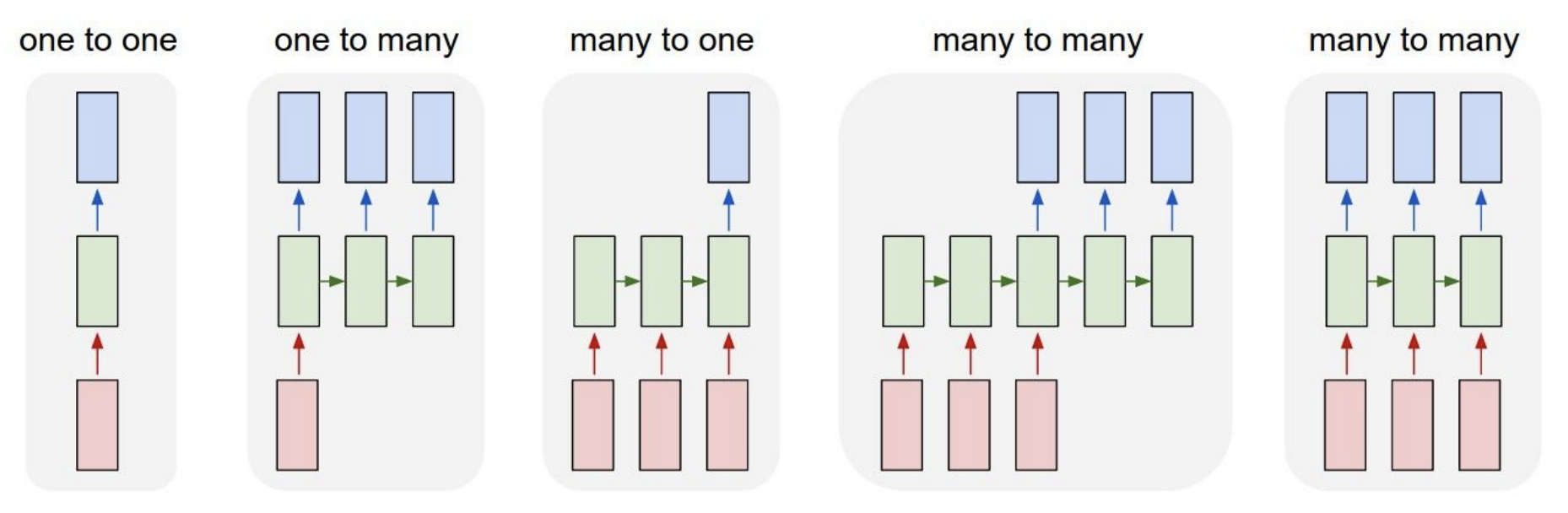Figure 1. Different (non-exhaustive) types of Recurrent Neural Network architectures. Red boxes are input vectors. Green boxes are hidden layers. Blue boxes are output vectors.

빨간 상자는 입력 벡터, 초록 상자는 은닉층, 파란 상자는 출력 벡터를 나타내며, 순환 신경망 구조에는 (여기 그린 것이 전부는 아니지만) 이렇게 다양한 유형이 있다.

Why are existing convnets insufficient?

The existing convnets are insufficient to deal with tasks that have inputs and outputs with variable sequence lengths. In the example of video captioning, inputs have variable number of frames (e.g. 10-minute and 10-hour long video) and outputs are captions of variable length. Convnets can only take in inputs with a fixed size of width and height and cannot generalize over inputs with different sizes. In order to tackle this problem, we introduce Recurrent Neural Networks (RNNs).

기존의 convnet은 입력과 출력의 시퀀스 길이가 가변적인 과제를 다루기에는 부족하다. 비디오 캡셔닝을 예로 들면, 입력은 프레임 수가 제각각이고(예컨대 10분짜리 비디오와 10시간짜리 비디오) 출력인 캡션도 길이가 제각각이다. convnet은 가로세로 크기가 고정된 입력만 받을 수 있어 크기가 다른 입력에는 일반화되지 않는다. 이 문제를 해결하기 위해 순환 신경망(RNN)을 도입한다.

Recurrent Neural Network

RNN is basically a blackbox (Left of Figure 2), where it has an “internal state” that is updated as a sequence is processed. At every single timestep, we feed in an input vector into RNN where it modifies that state as a function of what it receives. When we tune RNN weights, RNN will show different behaviors in terms of how its state evolves as it receives these inputs. We are also interested in producing an output based on the RNN state, so we can produce these output vectors on top of the RNN (as depicted in Figure 2).

RNN은 기본적으로 블랙박스(Figure 2의 왼쪽)로, 시퀀스가 처리되면서 갱신되는 “내부 상태”를 갖고 있다. 매 스텝마다 입력 벡터 하나를 RNN에 넣으면 RNN은 자신이 받은 것의 함수로 그 상태를 바꾼다. RNN의 가중치를 조정하면 RNN은 이 입력들을 받으면서 상태가 어떻게 변해 가는지에 있어 서로 다른 행동을 보인다. 또한 RNN의 상태를 바탕으로 출력을 만들어내는 데도 관심이 있으므로, RNN 위에 이 출력 벡터들을 만들어낼 수 있다(Figure 2에 그려진 대로).

If we unroll an RNN model (Right of Figure 2), then there are inputs (e.g. video frame) at different timesteps shown as \(x_1, x_2, x_3\) … \(x_t\). RNN at each timestep takes in two inputs – an input frame (\(x_i\)) and previous representation of what it seems so far (i.e. history) – to generate an output \(y_i\) and update its history, which will get forward propagated over time. All the RNN blocks in Figure 2 (Right) are the same block that share the same parameter, but have different inputs and history at each timestep.

RNN 모델을 펼치면(Figure 2의 오른쪽) 서로 다른 스텝의 입력들(예컨대 비디오 프레임)이 \(x_1, x_2, x_3\) … \(x_t\)로 나타난다. RNN은 매 스텝마다 입력 프레임(\(x_i\))과 지금까지 본 것을 나타내는 이전 표현(곧 이력)이라는 두 입력을 받아 출력 \(y_i\)를 만들어내고 자신의 이력을 갱신하며, 이 이력은 시간에 따라 순전파된다. Figure 2(오른쪽)의 RNN 블록은 모두 같은 매개변수를 공유하는 동일한 블록이지만, 스텝마다 입력과 이력이 다르다.

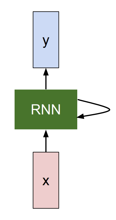
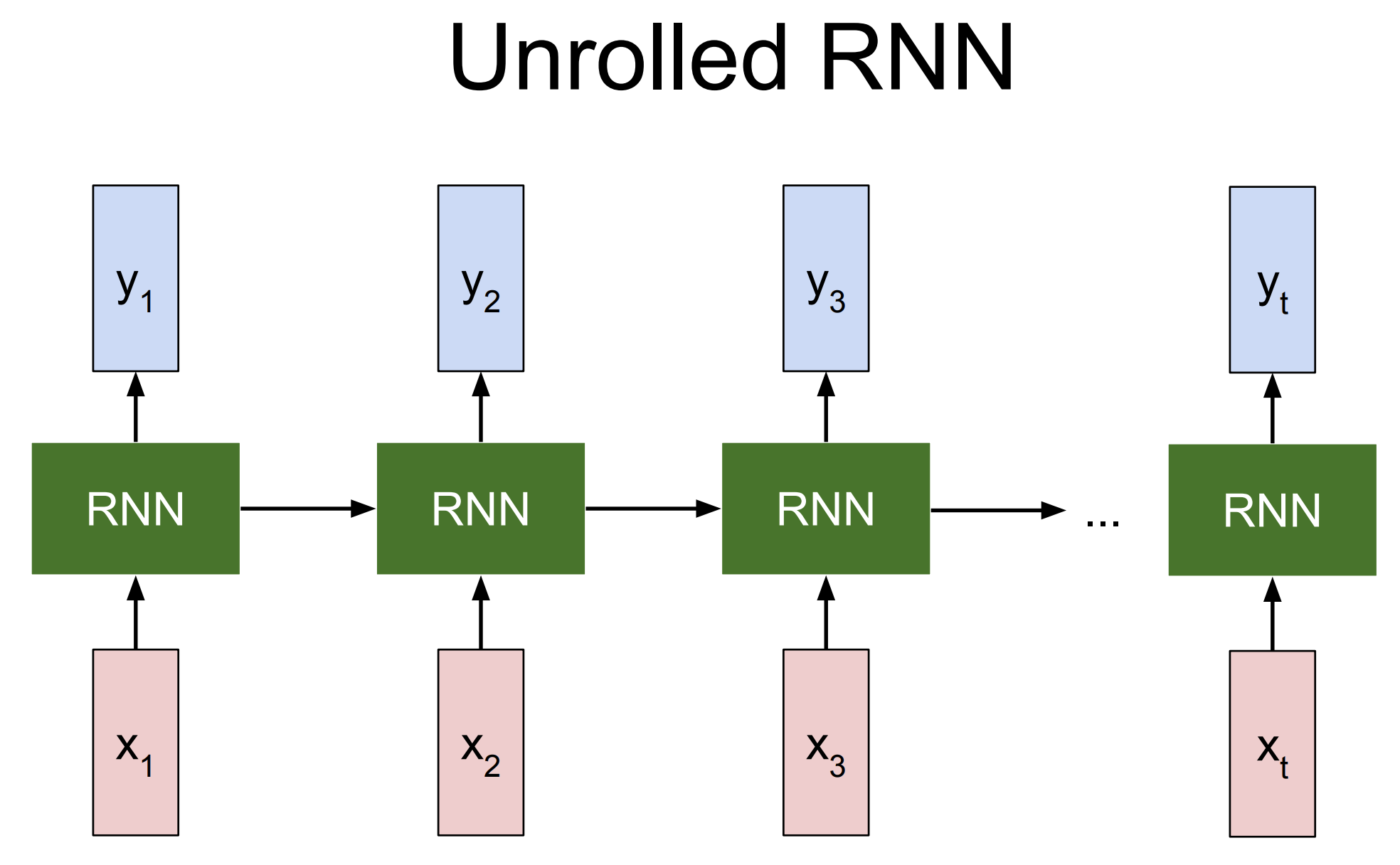Figure 2.Simplified RNN box (Left) and Unrolled RNN (Right).

단순화한 RNN 상자(왼쪽)와 그것을 펼친 RNN(오른쪽).

More precisely, RNN can be represented as a recurrence formula of some function \(f_W\) with parameters \(W\):

\[h_t = f_W(h_{t-1}, x_t)\]

더 정확히 말하면, RNN은 매개변수 \(W\)를 갖는 어떤 함수 \(f_W\)의 순환식(recurrence formula)으로 나타낼 수 있다.

where at every timestep it receives some previous state as a vector \(h_{t-1}\) of previous iteration timestep \(t-1\) and current input vector \(x_t\) to produce the current state as a vector \(h_t\). A fixed function \(f_W\) with weights \(W\) is applied at every single timestep and that allows us to use the Recurrent Neural Network on sequences without having to commit to the size of the sequence because we apply the exact same function at every single timestep, no matter how long the input or output sequences are.

여기서 매 스텝마다 이전 반복 스텝 \(t-1\)의 상태를 나타내는 벡터 \(h_{t-1}\)과 현재 입력 벡터 \(x_t\)를 받아 현재 상태를 나타내는 벡터 \(h_t\)를 만들어낸다. 가중치 \(W\)를 갖는 고정된 함수 \(f_W\)가 매 스텝마다 적용되는데, 이 덕분에 시퀀스의 길이를 미리 정해 두지 않고도 RNN을 시퀀스에 적용할 수 있다. 입력이나 출력 시퀀스가 아무리 길어도 매 스텝마다 정확히 같은 함수를 적용하기 때문이다.

역주. 여기서 “같은 함수 \(f_W\)“란 매 스텝마다 가중치를 새로 두지 않고 딱 한 벌의 가중치 \(W\)를 계속 재사용한다는 뜻이다. 예컨대 층마다 가중치가 다른 10층짜리 일반 신경망과 달리, RNN은 스텝이 10개든 1000개든 가중치 행렬의 크기는 그대로다. 그래서 학습 데이터에서 본 적 없는 길이의 시퀀스에도 같은 모델을 그대로 적용할 수 있다.

In the most simplest form of RNN, which we call a Vanilla RNN, the network is just a single hidden state \(h\) where we use a recurrence formula that basically tells us how we should update our hidden state \(h\) as a function of previous hidden state \(h_{t-1}\) and the current input \(x_t\). In particular, we’re going to have weight matrices \(W_{hh}\) and \(W_{xh}\), where they will project both the hidden state \(h_{t-1}\) from the previous timestep and the current input \(x_t\), and then those are going to be summed and squished with \(tanh\) function to update the hidden state \(h_t\) at timestep \(t\). This recurrence is telling us how \(h\) will change as a function of its history and also the current input at this timestep:

\[h_t = tanh(W_{hh}h_{t-1} + W_{xh}x_t)\]

RNN의 가장 단순한 형태, 곧 바닐라 RNN이라 부르는 것에서 신경망은 은닉 상태 \(h\) 하나로만 이루어져 있고, 이전 은닉 상태 \(h_{t-1}\)과 현재 입력 \(x_t\)의 함수로 은닉 상태 \(h\)를 어떻게 갱신할지 알려주는 순환식을 쓴다. 구체적으로는 가중치 행렬 \(W_{hh}\)와 \(W_{xh}\)를 두는데, 이 행렬들은 이전 스텝의 은닉 상태 \(h_{t-1}\)과 현재 입력 \(x_t\)를 각각 사영한 뒤 그 둘을 더하고 \(tanh\) 함수로 눌러 넣어 스텝 \(t\)의 은닉 상태 \(h_t\)를 갱신한다. 이 순환식은 \(h\)가 자신의 이력과 이 스텝의 현재 입력의 함수로 어떻게 변하는지 알려준다.

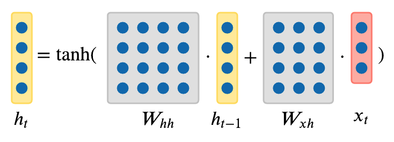
We can base predictions on top of \(h_t\) by using just another matrix projection on top of the hidden state. This is the simplest complete case in which you can wire up a neural network:

\[y_t = W_{hy}h_t\]

은닉 상태 위에 행렬 사영을 하나 더 적용해 \(h_t\)를 바탕으로 예측을 만들 수 있다. 이것이 신경망을 완전하게 구성할 수 있는 가장 단순한 경우다.

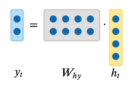
So far we have showed RNN in terms of abstract vectors \(x, h, y\), however we can endow these vectors with semantics in the following section.

지금까지는 RNN을 추상적인 벡터 \(x, h, y\)로 보여주었지만, 다음 절에서는 이 벡터들에 의미를 부여할 수 있다.

RNN example as Character-level language model

One of the simplest ways in which we can use an RNN is in the case of a character-level language model since it’s intuitive to understand. The way this RNN will work is we will feed a sequence of characters into the RNN and at every single timestep, we will ask the RNN to predict the next character in the sequence. The prediction of RNN will be in the form of score distribution of the characters in the vocabulary for what RNN thinks should come next in the sequence that it has seen so far.

RNN을 쓸 수 있는 가장 단순한 방법 가운데 하나는 직관적으로 이해하기 쉬운 문자 단위 언어 모델(character-level language model)의 경우다. 이 RNN이 동작하는 방식은, 문자의 시퀀스를 RNN에 입력으로 넣고 매 스텝마다 RNN에게 시퀀스의 다음 문자를 예측하게 하는 것이다. RNN의 예측은, 지금까지 본 시퀀스 다음에 무엇이 올지에 대해 RNN이 생각하는 바를 어휘(vocabulary)에 속한 문자들에 대한 점수 분포의 형태로 내놓는다.

So suppose, in a very simple example (Figure 3), we have the training sequence of just one string \(\text{"hello"}\), and we have a vocabulary \(V \in \{\text{"h"}, \text{"e"}, \text{"l"}, \text{"o"}\}\) of 4 characters in the entire dataset. We are going to try to get an RNN to learn to predict the next character in the sequence on this training data.

아주 단순한 예(Figure 3)를 들어, 학습 시퀀스가 문자열 \(\text{"hello"}\) 하나뿐이고 전체 데이터셋의 어휘가 4개 문자로 이루어진 \(V \in \{\text{"h"}, \text{"e"}, \text{"l"}, \text{"o"}\}\)라고 하자. 이 학습 데이터로 RNN이 시퀀스의 다음 문자를 예측하도록 학습시켜 볼 것이다.

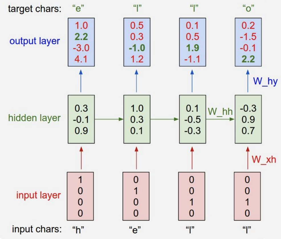Figure 3. Simplified Character-level Language Model RNN.

단순화한 문자 단위 언어 모델 RNN.

As shown in Figure 3, we’ll feed in one character at a time into an RNN, first \(\text{"h"}\), then \(\text{"e"}\), then \(\text{"l"}\), and finally \(\text{"l"}\). All characters are encoded in the representation of what’s called a one-hot vector, where only one unique bit of the vector is turned on for each unique character in the vocabulary. For example:

\[\begin{bmatrix}1 \\ 0 \\ 0 \\ 0 \end{bmatrix} = \text{"h"}\ \ \begin{bmatrix}0 \\ 1 \\ 0 \\ 0 \end{bmatrix} = \text{"e"}\ \ \begin{bmatrix}0 \\ 0 \\ 1 \\ 0 \end{bmatrix} = \text{"l"}\ \ \begin{bmatrix}0 \\ 0 \\ 0 \\ 1 \end{bmatrix} = \text{"o"}\]

Figure 3에서 보듯, RNN에 문자를 한 번에 하나씩, 먼저 \(\text{"h"}\), 그다음 \(\text{"e"}\), 그다음 \(\text{"l"}\), 마지막으로 \(\text{"l"}\)을 입력으로 넣는다. 모든 문자는 원-핫 벡터(one-hot vector)라는 표현으로 인코딩되는데, 여기서는 어휘의 문자마다 벡터에서 고유한 비트 하나만 켜진다. 예를 들면 다음과 같다.

Then we’re going to use the recurrence formula from the previous section at every single timestep. Suppose we start off with \(h\) as a vector of size 3 with all zeros. By using this fixed recurrence formula, we’re going to end up with a 3-dimensional representation of the next hidden state \(h\) that basically at any point in time summarizes all the characters that have come until then:

\[\begin{aligned} \begin{bmatrix}0.3 \\ -0.1 \\ 0.9 \end{bmatrix} &= f_W(W_{hh}\begin{bmatrix}0 \\ 0 \\ 0 \end{bmatrix} + W_{xh}\begin{bmatrix}1 \\ 0 \\ 0 \\ 0 \end{bmatrix}) \ \ \ \ &(1) \\ \begin{bmatrix}1.0 \\ 0.3 \\ 0.1 \end{bmatrix} &= f_W(W_{hh}\begin{bmatrix}0.3 \\ -0.1 \\ 0.9 \end{bmatrix} + W_{xh}\begin{bmatrix}0 \\ 1 \\ 0 \\ 0 \end{bmatrix}) \ \ \ \ &(2) \\ \begin{bmatrix}0.1 \\ -0.5 \\ -0.3 \end{bmatrix} &= f_W(W_{hh}\begin{bmatrix}1.0 \\ 0.3 \\ 0.1 \end{bmatrix} + W_{xh}\begin{bmatrix}0 \\ 0 \\ 1 \\ 0 \end{bmatrix}) \ \ \ \ &(3) \\ \begin{bmatrix}-0.3 \\ 0.9 \\ 0.7 \end{bmatrix} &= f_W(W_{hh}\begin{bmatrix}0.1 \\ -0.5 \\ -0.3 \end{bmatrix} + W_{xh}\begin{bmatrix}0 \\ 0 \\ 1 \\ 0 \end{bmatrix}) \ \ \ \ &(4) \end{aligned}\]

그다음에는 앞 절의 순환식을 매 스텝마다 적용한다. 처음에 \(h\)를 크기 3인 벡터로 두고 모든 값을 0으로 시작한다고 하자. 이 고정된 순환식을 적용하면, 어느 시점에서든 그때까지 나온 문자들을 요약해 주는 다음 은닉 상태 \(h\)의 3차원 표현을 얻게 된다.

As we apply this recurrence at every timestep, we’re going to predict what should be the next character in the sequence at every timestep. Since we have four characters in vocabulary \(V\), we’re going to predict 4-dimensional vector of logits at every single timestep.

이 순환식을 매 스텝마다 적용하면서 시퀀스에서 다음에 와야 할 문자가 무엇인지 매 스텝마다 예측한다. 어휘 \(V\)에 네 개의 문자가 있으므로, 매 스텝마다 4차원 logit 벡터를 예측하게 된다.

As shown in Figure 3, in the very first timestep we fed in \(\text{"h"}\), and the RNN with its current setting of weights computed a vector of logits:

\[\begin{bmatrix}1.0 \\ 2.2 \\ -3.0 \\ 4.1 \end{bmatrix} \rightarrow \begin{bmatrix}\text{"h"} \\ \text{"e"} \\ \text{"l"}\\ \text{"o"} \end{bmatrix}\]

Figure 3에서 보듯, 아주 첫 번째 스텝에서 \(\text{"h"}\)를 입력으로 넣었고, 현재 가중치 값을 가진 RNN은 다음과 같은 logit 벡터를 계산했다.

where RNN thinks that the next character \(\text{"h"}\) is \(1.0\) likely to come next, \(\text{"e"}\) is \(2.2\) likely, \(\text{"e"}\) is \(-3.0\) likely, and \(\text{"o"}\) is \(4.1\) likely to come next. In this case, RNN incorrectly suggests that \(\text{"o"}\) should come next, as the score of \(4.1\) is the highest. However, of course, we know that in this training sequence \(\text{"e"}\) should follow \(\text{"h"}\), so in fact the score of \(2.2\) is the correct answer as it’s highlighted in green in Figure 3, and we want that to be high and all other scores to be low. At every single timestep we have a target for what next character should come in the sequence, therefore the error signal is backpropagated as a gradient of the loss function through the connections. As a loss function we could choose to have a softmax classifier, for example, so we just get all those losses flowing down from the top backwards to calculate the gradients on all the weight matrices to figure out how to shift the matrices so that the correct probabilities are coming out of the RNN. Similarly we can imagine how to scale up the training of the model over larger training dataset.

여기서 RNN은 다음 문자로 \(\text{"h"}\)가 나올 가능성을 \(1.0\), \(\text{"e"}\)를 \(2.2\), \(\text{"e"}\)를 \(-3.0\), \(\text{"o"}\)를 \(4.1\)로 본다. 이 경우 점수 \(4.1\)이 가장 높으므로 RNN은 다음에 \(\text{"o"}\)가 와야 한다고 잘못 판단한 것이다. 그러나 물론 이 학습 시퀀스에서는 \(\text{"h"}\) 다음에 \(\text{"e"}\)가 와야 한다는 것을 우리는 알고 있으므로, 사실은 Figure 3에서 초록색으로 강조된 점수 \(2.2\)가 정답이며 이 값은 높이고 나머지 점수는 모두 낮추고 싶다. 매 스텝마다 시퀀스에서 다음에 와야 할 문자에 대한 목표값이 있으므로, 오차 신호는 손실 함수의 기울기로서 연결을 통해 역전파된다. 손실 함수로는 예컨대 softmax 분류기를 선택할 수 있고, 그러면 이 손실들이 맨 위에서부터 거꾸로 흘러 내려가면서 모든 가중치 행렬에 대한 기울기를 계산해, RNN에서 올바른 확률이 나오도록 행렬을 어떻게 옮겨야 할지 알아낸다. 마찬가지로 이 모델의 학습을 더 큰 학습 데이터셋으로 어떻게 확장할지도 상상해 볼 수 있다.

Multilayer RNNs

So far we have only shown RNNs with just one layer. However, we’re not limited to only a single layer architectures. One of the ways, RNNs are used today is in more complex manner. RNNs can be stacked together in multiple layers, which gives more depth, and empirically deeper architectures tend to work better (Figure 4).

지금까지는 층이 하나뿐인 RNN만 보여주었다. 그렇지만 단일 층 구조에만 한정되는 것은 아니다. 오늘날 RNN이 쓰이는 방식 가운데 하나는 더 복잡한 형태다. RNN을 여러 층으로 쌓아 올릴 수 있으며, 이는 더 큰 깊이를 주고 경험적으로 더 깊은 구조가 더 잘 작동하는 경향이 있다(Figure 4).

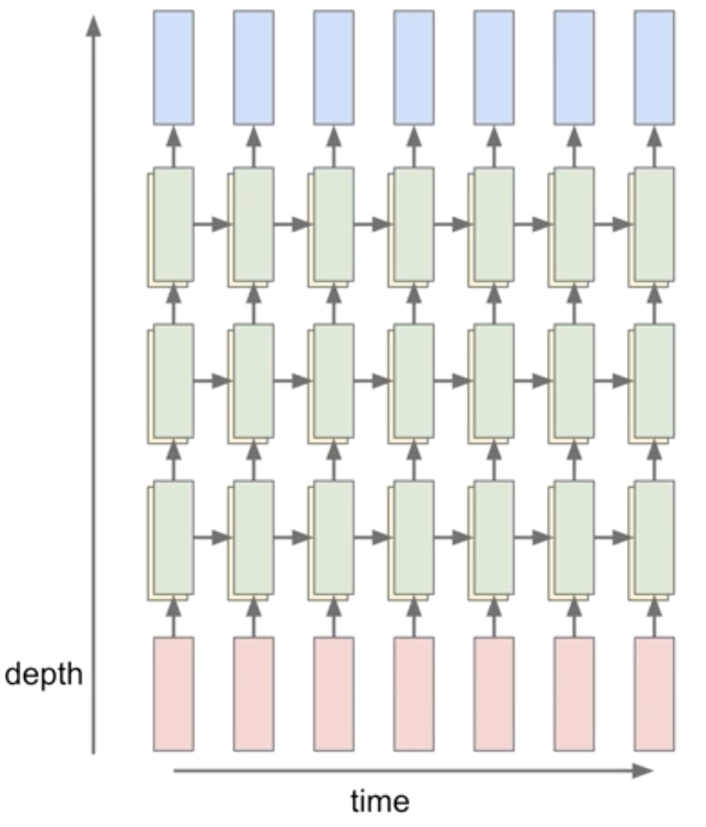Figure 4. Multilayer RNN example.

다층 RNN의 예.

For example, in Figure 4, there are three separate RNNs each with their own set of weights. Three RNNs are stacked on top of each other, so the input of the second RNN (second RNN layer in Figure 4) is the vector of the hidden state vector of the first RNN (first RNN layer in Figure 4). All stacked RNNs are trained jointly, and the diagram in Figure 4 represents one computational graph.

예컨대 Figure 4에는 각자 자기만의 가중치 집합을 가진 별개의 RNN 세 개가 있다. 이 세 RNN은 서로 위로 쌓여 있어서, 두 번째 RNN(Figure 4의 두 번째 RNN 층)의 입력은 첫 번째 RNN(Figure 4의 첫 번째 RNN 층)의 은닉 상태 벡터가 된다. 쌓아 올린 RNN들은 함께 학습되며, Figure 4의 도식은 하나의 계산 그래프를 나타낸다.

Long-Short Term Memory (LSTM)

So far we have seen only a simple recurrence formula for the Vanilla RNN. In practice, we actually will rarely ever use Vanilla RNN formula. Instead, we will use what we call a Long-Short Term Memory (LSTM) RNN.

지금까지는 바닐라 RNN에 대한 단순한 순환식만 살펴보았다. 실제로는 바닐라 RNN 식을 그대로 쓰는 일이 거의 없다. 그 대신 Long-Short Term Memory(LSTM) RNN이라 부르는 것을 쓴다.

Vanilla RNN Gradient Flow & Vanishing Gradient Problem

An RNN block takes in input \(x_t\) and previous hidden representation \(h_{t-1}\) and learn a transformation, which is then passed through tanh to produce the hidden representation \(h_{t}\) for the next time step and output \(y_{t}\) as shown in the equation below.

\[h_t = tanh(W_{hh}h_{t-1} + W_{xh}x_t)\]

RNN 블록은 입력 \(x_t\)와 이전 은닉 표현 \(h_{t-1}\)을 받아 어떤 변환을 학습하고, 그 결과를 tanh에 통과시켜 아래 식처럼 다음 스텝을 위한 은닉 표현 \(h_{t}\)와 출력 \(y_{t}\)를 만들어낸다.

For the back propagation, Let’s examine how the output at the very last timestep affects the weights at the very first time step. The partial derivative of \(h_t\) with respect to \(h_{t-1}\) is written as: \(\frac{\partial h_t}{\partial h_{t-1}} = tanh^{'}(W_{hh}h_{t-1} + W_{xh}x_t)W_{hh}\)

역전파를 위해, 아주 마지막 스텝의 출력이 아주 첫 번째 스텝의 가중치에 어떤 영향을 미치는지 살펴보자. \(h_{t-1}\)에 대한 \(h_t\)의 편미분은 다음과 같이 쓸 수 있다. \(\frac{\partial h_t}{\partial h_{t-1}} = tanh^{'}(W_{hh}h_{t-1} + W_{xh}x_t)W_{hh}\)

We update the weights \(W_{hh}\) by getting the derivative of the loss at the very last time step \(L_{t}\) with respect to \(W_{hh}\).

\[\begin{aligned} \frac{\partial L_{t}}{\partial W_{hh}} = \frac{\partial L_{t}}{\partial h_{t}} \frac{\partial h_{t}}{\partial h_{t-1} } \dots \frac{\partial h_{1}}{\partial W_{hh}} \\ = \frac{\partial L_{t}}{\partial h_{t}}(\prod_{t=2}^{T} \frac{\partial h_{t}}{\partial h_{t-1}})\frac{\partial h_{1}}{\partial W_{hh}} \\ = \frac{\partial L_{t}}{\partial h_{t}}(\prod_{t=2}^{T} tanh^{'}(W_{hh}h_{t-1} + W_{xh}x_t)W_{hh}^{T-1})\frac{\partial h_{1}}{\partial W_{hh}} \\ \end{aligned}\]

가중치 \(W_{hh}\)는 아주 마지막 스텝의 손실 \(L_{t}\)를 \(W_{hh}\)에 대해 미분해 얻은 값으로 갱신한다.

• Vanishing gradient: We see that \(tanh^{'}(W_{hh}h_{t-1} + W_{xh}x_t)\) will almost always be less than 1 because tanh is always between negative one and one. Thus, as \(t\) gets larger (i.e. longer timesteps), the gradient (\(\frac{\partial L_{t}}{\partial W}\)) will descrease in value and get close to zero. This will lead to vanishing gradient problem, where gradients at future time steps rarely impact gradients at the very first time step. This is problematic when we model long sequence of inputs because the updates will be extremely slow.
• Removing non-linearity (tanh): If we remove non-linearity (tanh) to solve the vanishing gradient problem, then we will be left with \(\begin{aligned} \frac{\partial L_{t}}{\partial W} = \frac{\partial L_{t}}{\partial h_{t}}(\prod_{t=2}^{T} W_{hh}^{T-1})\frac{\partial h_{1}}{\partial W} \end{aligned}\)
• Exploding gradients: If the largest singular value of W_{hh} is greater than 1, then the gradients will blow up and the model will get very large gradients coming back from future time steps. Exploding gradient often leads to getting gradients that are NaNs.
• Vanishing gradients: If the laregest singular value of W_{hh} is smaller than 1, then we will have vanishing gradient problem as mentioned above which will significantly slow down learning.

• 기울기 소실(Vanishing gradient): \(tanh^{'}(W_{hh}h_{t-1} + W_{xh}x_t)\)은 tanh 값이 항상 -1과 1 사이에 있기 때문에 거의 언제나 1보다 작다. 따라서 \(t\)가 커질수록(곧 스텝이 길어질수록) 기울기(\(\frac{\partial L_{t}}{\partial W}\))의 값은 점점 작아져 0에 가까워진다. 이는 기울기 소실 문제로 이어지는데, 이후 스텝의 기울기가 아주 첫 번째 스텝의 기울기에 거의 영향을 미치지 못하게 된다. 긴 입력 시퀀스를 모델링할 때는 갱신이 극도로 느려지므로 이것이 문제가 된다.
• 비선형성(tanh) 제거하기(Removing non-linearity (tanh)): 기울기 소실 문제를 풀려고 비선형성(tanh)을 제거하면 다음 식만 남는다. \(\begin{aligned} \frac{\partial L_{t}}{\partial W} = \frac{\partial L_{t}}{\partial h_{t}}(\prod_{t=2}^{T} W_{hh}^{T-1})\frac{\partial h_{1}}{\partial W} \end{aligned}\)
• 기울기 폭발(exploding gradient): \(W_{hh}\)의 가장 큰 특잇값이 1보다 크면 기울기가 폭발하듯 커져서, 모델은 이후 스텝들로부터 거꾸로 아주 큰 기울기를 받게 된다. 기울기가 폭발하면 흔히 기울기 값이 NaN이 되어 버린다.
• 기울기 소실: \(W_{hh}\)의 가장 큰 특잇값이 1보다 작으면 앞서 말한 기울기 소실 문제가 생겨 학습이 크게 느려진다.

In practice, we can treat the exploding gradient problem through gradient clipping, which is clipping large gradient values to a maximum threshold. However, since vanishing gradient problem still exists in cases where largest singular value of W_{hh} matrix is less than one, LSTM was designed to avoid this problem.

실무에서는 기울기 폭발 문제를 기울기 클리핑(gradient clipping)으로 다룰 수 있는데, 이는 큰 기울기 값을 어떤 최대 문턱값으로 잘라내는 것이다. 그러나 \(W_{hh}\) 행렬의 가장 큰 특잇값이 1보다 작은 경우에는 기울기 소실 문제가 여전히 남아 있으므로, 이 문제를 피하기 위해 LSTM이 고안되었다.

역주. 기울기 클리핑이 기울기 폭발만 고칠 수 있고 기울기 소실은 고치지 못하는 이유는 두 문제의 방향이 다르기 때문이다. 클리핑은 기울기 값에 위쪽 한계를 씌우는 연산이라, 너무 커진 값을 깎아내리는 데는 쓸 수 있지만 이미 0에 가까워진 값을 다시 키워주지는 못한다. 즉 클리핑은 천장은 낮출 수 있어도 바닥을 들어 올리지는 못하며, 기울기 소실은 바닥이 꺼지는 문제이므로 클리핑으로는 손댈 수 없다. LSTM은 이 바닥 쪽 문제, 곧 기울기 소실을 겨냥해 고안되었다.

LSTM Formulation

The following is the precise formulation for LSTM. On step \(t\), there is a hidden state \(h_t\) and a cell state \(c_t\). Both \(h_t\) and \(c_t\) are vectors of size \(n\). One distinction of LSTM from Vanilla RNN is that LSTM has this additional \(c_t\) cell state, and intuitively it can be thought of as \(c_t\) stores long-term information. LSTM can read, erase, and write information to and from this \(c_t\) cell. The way LSTM alters \(c_t\) cell is through three special gates: \(i, f, o\) which correspond to “input”, “forget”, and “output” gates. The values of these gates vary from closed (0) to open (1). All \(i, f, o\) gates are vectors of size \(n\).

다음은 LSTM의 정확한 정의다. 스텝 \(t\)에는 은닉 상태 \(h_t\)와 셀 상태(cell state) \(c_t\)가 있다. \(h_t\)와 \(c_t\) 모두 크기 \(n\)인 벡터다. LSTM이 바닐라 RNN과 다른 점 하나는 이렇게 셀 상태 \(c_t\)가 추가로 있다는 것인데, 직관적으로 \(c_t\)는 장기적인 정보를 저장한다고 볼 수 있다. LSTM은 이 \(c_t\) 셀에 정보를 읽고, 지우고, 쓸 수 있다. LSTM이 \(c_t\) 셀을 바꾸는 방식은 “input”, “forget”, “output” 게이트에 대응하는 \(i, f, o\)라는 세 개의 특수한 게이트를 통해서다. 이 게이트들의 값은 닫힘(0)에서 열림(1)까지 다양하다. \(i, f, o\) 게이트는 모두 크기 \(n\)인 벡터다.

At every timestep we have an input vector \(x_t\), previous hidden state \(h_{t-1}\), previous cell state \(c_{t-1}\), and LSTM computes the next hidden state \(h_t\), and next cell state \(c_t\) at timestep \(t\) as follows:

\[\begin{aligned} f_t &= \sigma(W_{hf}h_{t_1} + W_{xf}x_t) \\ i_t &= \sigma(W_{hi}h_{t_1} + W_{xi}x_t) \\ o_t &= \sigma(W_{ho}h_{t_1} + W_{xo}x_t) \\ g_t &= \text{tanh}(W_{hg}h_{t_1} + W_{xg}x_t) \\ \end{aligned}\]

매 스텝마다 입력 벡터 \(x_t\), 이전 은닉 상태 \(h_{t-1}\), 이전 셀 상태 \(c_{t-1}\)이 있고, LSTM은 다음과 같이 스텝 \(t\)의 다음 은닉 상태 \(h_t\)와 다음 셀 상태 \(c_t\)를 계산한다.

\[\begin{aligned} c_t &= f_t \odot c_{t-1} + i_t \odot g_t \\ h_t &= o_t \odot \text{tanh}(c_t) \\ \end{aligned}\]

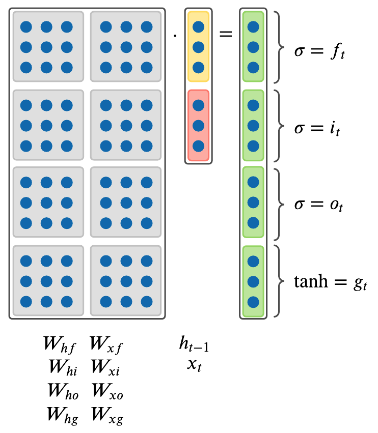
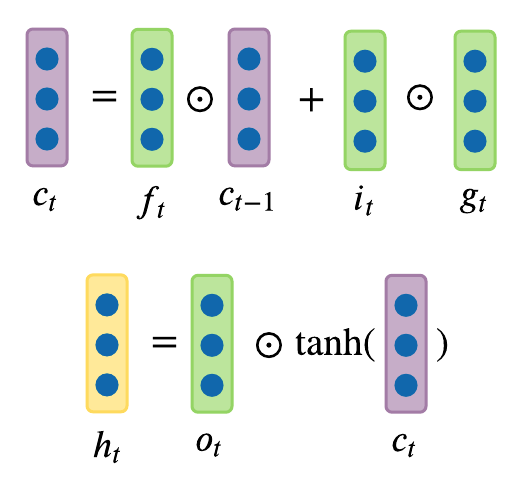
where \(\odot\) is an element-wise Hadamard product. \(g_t\) in the above formulas is an intermediary calculation cache that’s later used with \(o\) gate in the above formulas.

여기서 \(\odot\)은 원소별 아다마르 곱(Hadamard product)이다. 위 식의 \(g_t\)는 나중에 \(o\) 게이트와 함께 쓰이는 중간 계산 캐시다.

역주. \(g_t\)가 “gate” 게이트라는 다소 헷갈리는 이름으로 불리지만, 정작 sigmoid가 아니라 tanh를 쓴다는 점에서 \(f, i, o\)와는 성격이 다르다. 다른 자료에서는 흔히 \(g_t\)를 후보 셀 상태(candidate cell state, 흔히 \(\tilde{c}_t\)로 표기)라고 부른다. 실제로 값을 0과 1 사이로 열고 닫는 진짜 게이트는 \(f, i, o\) 셋뿐이고, \(g_t\)는 그 게이트들이 걸러낼 “새로 셀에 넣을 후보 값”을 만드는 역할이다. 참고로 바로 위 원문은 \(g_t\)가 나중에 \(o\) 게이트와 함께 쓰인다고 적었지만, 그 위 수식 \(c_t = f_t \odot c_{t-1} + i_t \odot g_t\)를 보면 실제로 \(g_t\)와 결합되는 것은 \(i\) 게이트이고 \(o\)는 \(c_t\)를 \(h_t\)로 내보낼 때만 쓰인다 — 원문 자체의 오류이며, 번역은 원문을 그대로 옮겼다.

Since all \(f, i, o\) gate vector values range from 0 to 1, because they were squashed by sigmoid function \(\sigma\), when multiplied element-wise, we can see that:

\(f, i, o\) 게이트 벡터의 값은 모두 sigmoid 함수 \(\sigma\)로 눌러 넣어졌기 때문에 0에서 1 사이의 범위를 가지며, 이 값들을 원소별로 곱하면 다음을 알 수 있다.

• Forget Gate: Forget gate \(f_t\) at time step \(t\) controls how much information needs to be “removed” from the previous cell state \(c_{t-1}\). This forget gate learns to erase hidden representations from the previous time steps, which is why LSTM will have two hidden represtnations \(h_t\) and cell state \(c_t\). This \(c_t\) will get propagated over time and learn whether to forget the previous cell state or not.
• Input Gate: Input gate \(i_t\) at time step \(t\) controls how much information needs to be “added” to the next cell state \(c_t\) from previous hidden state \(h_{t-1}\) and input \(x_t\). Instead of tanh, the “input” gate \(i\) has a sigmoid function, which converts inputs to values between zero and one. This serves as a switch, where values are either almost always zero or almost always one. This “input” gate decides whether to take the RNN output that is produced by the “gate” gate \(g\) and multiplies the output with input gate \(i\).
• Output Gate: Output gate \(o_t\) at time step \(t\) controls how much information needs to be “shown” as output in the current hidden state \(h_t\).

• Forget 게이트: 스텝 \(t\)의 forget 게이트 \(f_t\)는 이전 셀 상태 \(c_{t-1}\)에서 얼마만큼의 정보를 “제거”해야 하는지 조절한다. 이 forget 게이트는 이전 스텝들의 은닉 표현을 지우는 법을 학습하는데, 이것이 바로 LSTM이 은닉 표현 \(h_t\)와 셀 상태 \(c_t\) 두 가지를 갖는 이유다. 이 \(c_t\)는 시간에 따라 전파되면서 이전 셀 상태를 잊을지 말지를 학습한다.
• Input 게이트: 스텝 \(t\)의 input 게이트 \(i_t\)는 이전 은닉 상태 \(h_{t-1}\)과 입력 \(x_t\)로부터 다음 셀 상태 \(c_t\)에 얼마만큼의 정보를 “추가”해야 하는지 조절한다. tanh 대신 “input” 게이트 \(i\)는 sigmoid 함수를 가지는데, 이는 입력을 0과 1 사이의 값으로 바꾼다. 이는 값이 거의 언제나 0이거나 거의 언제나 1인 스위치 역할을 한다. 이 “input” 게이트는 “gate” 게이트 \(g\)가 만들어내는 RNN 출력을 취할지 말지를 결정하고, 그 출력을 input 게이트 \(i\)와 곱한다.
• Output 게이트: 스텝 \(t\)의 output 게이트 \(o_t\)는 현재 은닉 상태 \(h_t\)에서 얼마만큼의 정보를 출력으로 “보여줘야” 하는지 조절한다.

The key idea of LSTM is the cell state, the horizontal line running through between recurrent timesteps. You can imagine the cell state to be some kind of highway of information passing through straight down the entire chain, with only some minor linear interactions. With the formulation above, it’s easy for information to just flow along this highway (Figure 5). Thus, even when there is a bunch of LSTMs stacked together, we can get an uninterrupted gradient flow where the gradients flow back through cell states instead of hidden states \(h\) without vanishing in every time step.

LSTM의 핵심 아이디어는 셀 상태, 곧 순환하는 스텝들 사이를 관통해 지나가는 가로줄이다. 셀 상태는 전체 사슬을 따라 곧장 흘러가는 일종의 정보 고속도로라고 생각할 수 있는데, 이 고속도로에는 몇 가지 사소한 선형 상호작용만 일어난다. 위의 정의를 따르면 정보가 이 고속도로를 따라 그대로 흘러가기 쉽다(Figure 5). 그래서 LSTM을 여러 개 쌓아 올려도, 기울기가 매 스텝마다 소실되지 않은 채 은닉 상태 \(h\)가 아니라 셀 상태를 거쳐 거꾸로 흐르는, 끊기지 않는 기울기 흐름을 얻을 수 있다.

역주. 왜 이 경로가 기울기를 소실시키지 않는지는 셀 상태의 재귀식 \(c_t = f_t \odot c_{t-1} + i_t \odot g_t\)을 \(c_{t-1}\)로 미분해 보면 바로 드러난다. \(\frac{\partial c_t}{\partial c_{t-1}} = f_t\)로, 바닐라 RNN의 \(\frac{\partial h_t}{\partial h_{t-1}} = tanh^{'}(\cdots)W_{hh}\)처럼 \(tanh^{'}\)과 가중치 행렬이 곱해지는 항이 아니라 forget 게이트 값 그 자체다. forget 게이트가 1에 가깝게 학습되면 이 미분값도 1에 가까워서, 여러 스텝을 거슬러 곱해도 값이 잘 줄어들지 않는다. 셀 상태가 “고속도로”인 이유가 바로 이 지점이다.

This greatly fixes the gradient vanishing/exploding problem we have outlined above. Figure 5 also shows that gradient contains a vector of activations of the “forget” gate. This allows better control of gradients values by using suitable parameter updates of the “forget” gate.

이는 앞서 설명한 기울기 소실/폭발 문제를 크게 해결해 준다. Figure 5는 또한 기울기가 “forget” 게이트의 활성값 벡터를 포함하고 있음을 보여준다. 이 덕분에 “forget” 게이트의 매개변수를 적절히 갱신함으로써 기울기 값을 더 잘 조절할 수 있다.

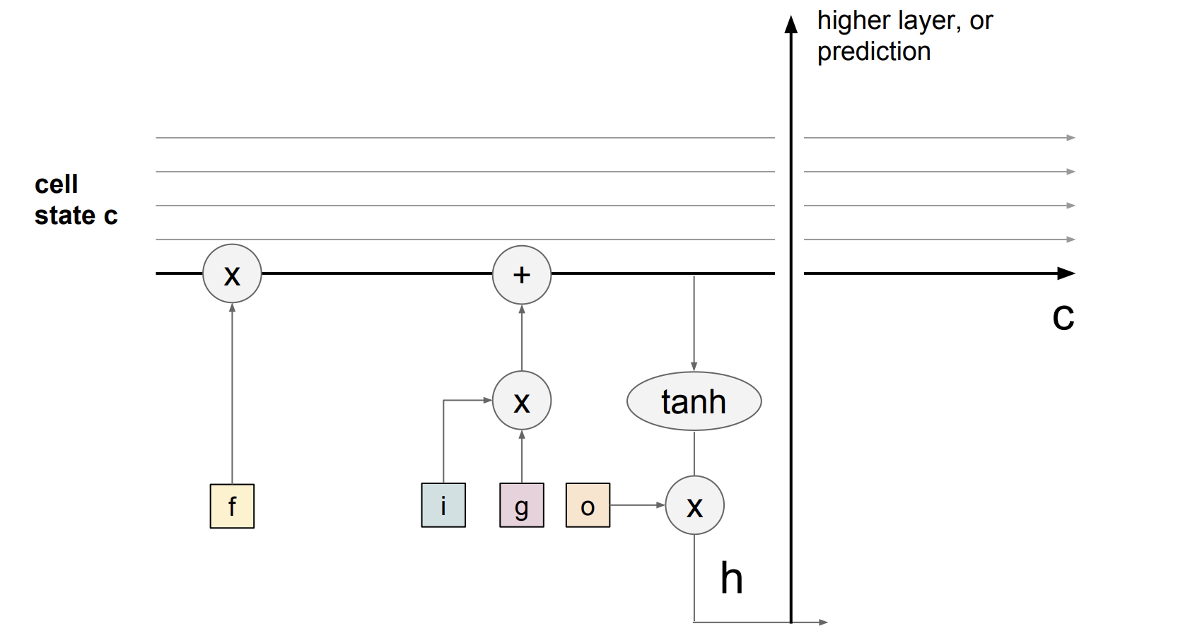Figure 5. LSTM cell state highway.

LSTM의 셀 상태 고속도로.

보충: 스텝 수에 따른 기울기 곱의 크기 변화

앞서 본 것처럼 바닐라 RNN의 기울기에는 \(tanh^{'}(\cdots)W_{hh}\)가 스텝마다 곱해지고, LSTM의 셀 상태 경로에는 forget 게이트 값이 곱해진다. 두 경우 모두 “1보다 작은 값을 T번 곱하면 T가 커질수록 얼마나 작아지는가”의 문제이므로, 그 크기만 따로 떼어 계산해 보면 감이 잡힌다. 바닐라 쪽은 0.6을, LSTM 쪽은 forget 게이트가 0.95 그리고 1로 학습된 두 경우를 비교했다.

steps = [5, 10, 20, 50, 100]

# 바닐라 RNN 쪽 factor: tanh'(*) * ||W_hh|| 를 대표하는 상수. tanh' < 1 이고
# ||W_hh|| 도 1에 가깝다고 가정하면 곱은 1보다 살짝 작은 값이 되기 쉽다.
vanilla_factor = 0.6

# LSTM 쪽 factor: forget 게이트 값. 학습이 "이 정보는 계속 들고 가라"고
# 판단하면 1에 가까운 값으로 수렴한다.
lstm_factor_high = 0.95
lstm_factor_perfect = 1.0

print(f"{'T':>4} | {'0.6^T (바닐라 근사)':>20} | {'0.95^T (forget=0.95)':>22} | {'1.0^T (forget=1)':>18}")
for T in steps:
    v = vanilla_factor ** T
    l = lstm_factor_high ** T
    p = lstm_factor_perfect ** T
    print(f"{T:>4} | {v:20.6g} | {l:22.6g} | {p:18.6g}")

실행 결과($WORK/.venv/bin/python):

   T |       0.6^T (바닐라 근사) |   0.95^T (forget=0.95) |   1.0^T (forget=1)
   5 |              0.07776 |               0.773781 |                  1
  10 |           0.00604662 |               0.598737 |                  1
  20 |          3.65616e-05 |               0.358486 |                  1
  50 |          8.08281e-12 |               0.076945 |                  1
 100 |          6.53319e-23 |             0.00592053 |                  1

바닐라 쪽은 스텝 20만 지나도 사실상 0으로 사라지지만, forget 게이트가 0.95인 LSTM 경로는 스텝 100에서도 0.006 정도로 완만하게 줄어들 뿐이고, forget 게이트를 1로 학습했다면 아예 줄어들지 않는다. 물론 이건 두 곱셈 인자만 단순화해 비교한 것이고, 실제 바닐라 RNN의 \(tanh^{'}(\cdots)W_{hh}\)는 매 스텝 값이 달라지며 행렬이므로 이보다 훨씬 복잡하게 움직인다. 그래도 “1보다 작은 값을 반복해서 곱하면 지수적으로 작아진다”는 핵심은 그대로 남는다.

Does LSTM solve the vanishing gradient problem?

LSTM architecture makes it easier for the RNN to preserve information over many recurrent time steps. For example, if the forget gate is set to 1, and the input gate is set to 0, then the infomation of the cell state will always be preserved over many recurrent time steps. For a Vanilla RNN, in contrast, it’s much harder to preserve information in hidden states in recurrent time steps by just making use of a single weight matrix.

LSTM 구조는 RNN이 여러 순환 스텝에 걸쳐 정보를 보존하기 더 쉽게 만들어준다. 예컨대 forget 게이트를 1로, input 게이트를 0으로 두면 셀 상태의 정보는 여러 순환 스텝에 걸쳐 항상 그대로 보존된다. 이와 달리 바닐라 RNN에서는 가중치 행렬 하나만으로 순환 스텝에 걸쳐 은닉 상태의 정보를 보존하기가 훨씬 더 어렵다.

LSTMs do not guarantee that there is no vanishing/exploding gradient problems, but it does provide an easier way for the model to learn long-distance dependencies.

LSTM이 기울기 소실/폭발 문제가 전혀 없다고 보장하지는 않지만, 모델이 장거리 의존성을 학습할 수 있는 더 쉬운 방법을 제공하는 것은 맞다.