01. Image Classification: Data-driven Approach, k-Nearest Neighbor, train/val/test splits

원문: Image Classification: Data-driven Approach, k-Nearest Neighbor, train/val/test splits — CS231n: Convolutional Neural Networks for Visual Recognition (Stanford University) · © 2015 Andrej Karpathy, MIT License

원문을 문단 단위로 인용하고 그 아래에 한국어 번역을 붙였다. 인용 블록이 원문, 그 아래 문단이 번역이며, 역주 박스와 보충 섹션은 원문에 없는 추가 내용이다.

This is an introductory lecture designed to introduce people from outside of Computer Vision to the Image Classification problem, and the data-driven approach. The Table of Contents:

컴퓨터 비전을 처음 접하는 사람에게 이미지 분류(image classification) 문제와 데이터 기반 접근법을 소개하는 입문 강의다. 목차는 다음과 같다.

• Image Classification
• Nearest Neighbor Classifier
• k - Nearest Neighbor Classifier
• Validation sets for Hyperparameter tuning
• Summary
• Summary: Applying kNN in practice
• Further Reading

• 이미지 분류
• 최근접 이웃 분류기
• k-최근접 이웃 분류기
• 하이퍼파라미터 튜닝을 위한 검증 집합
• 정리
• 정리: kNN을 실제로 적용하기
• 더 읽을거리

Image Classification

Motivation. In this section we will introduce the Image Classification problem, which is the task of assigning an input image one label from a fixed set of categories. This is one of the core problems in Computer Vision that, despite its simplicity, has a large variety of practical applications. Moreover, as we will see later in the course, many other seemingly distinct Computer Vision tasks (such as object detection, segmentation) can be reduced to image classification.

동기(Motivation). 이 절에서는 이미지 분류 문제를 소개한다. 고정된 카테고리 집합에서 레이블 하나를 골라 입력 이미지에 할당하는 작업이다. 컴퓨터 비전의 핵심 문제 가운데 하나로, 단순해 보이지만 실제 응용 범위는 대단히 넓다. 게다가 뒤에서 보겠지만 물체 검출(object detection)이나 분할(segmentation)처럼 겉보기에는 전혀 달라 보이는 컴퓨터 비전 과제도 상당수가 이미지 분류로 환원된다.

Example. For example, in the image below an image classification model takes a single image and assigns probabilities to 4 labels, {cat, dog, hat, mug}. As shown in the image, keep in mind that to a computer an image is represented as one large 3-dimensional array of numbers. In this example, the cat image is 248 pixels wide, 400 pixels tall, and has three color channels Red,Green,Blue (or RGB for short). Therefore, the image consists of 248 x 400 x 3 numbers, or a total of 297,600 numbers. Each number is an integer that ranges from 0 (black) to 255 (white). Our task is to turn this quarter of a million numbers into a single label, such as “cat”.

예시(Example). 아래 그림에서 이미지 분류 모델은 이미지 한 장을 받아 {cat, dog, hat, mug} 네 개 레이블에 확률을 매긴다. 그림에서 보듯 컴퓨터에게 이미지란 커다란 3차원 숫자 배열 하나라는 점을 기억해두자. 이 예시의 고양이 이미지는 너비 248픽셀, 높이 400픽셀이고 빨강, 초록, 파랑(줄여서 RGB) 세 개의 색 채널을 가진다. 따라서 이 이미지는 248 x 400 x 3개, 모두 297,600개의 숫자로 이루어진다. 각 숫자는 0(검정)부터 255(흰색)까지의 정수다. 우리가 할 일은 이 25만 개 남짓한 숫자를 “고양이”라는 레이블 하나로 바꾸는 것이다.

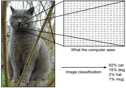The task in Image Classification is to predict a single label (or a distribution over labels as shown here to indicate our confidence) for a given image. Images are 3-dimensional arrays of integers from 0 to 255, of size Width x Height x 3. The 3 represents the three color channels Red, Green, Blue.

이미지 분류의 과제는 주어진 이미지에 대해 레이블 하나를, 혹은 그림처럼 확신도를 나타내는 레이블 분포를 예측하는 것이다. 이미지는 너비 x 높이 x 3 크기이고 0부터 255까지의 정수로 이루어진 3차원 배열이다. 여기서 3은 빨강, 초록, 파랑 세 개의 색 채널을 뜻한다.

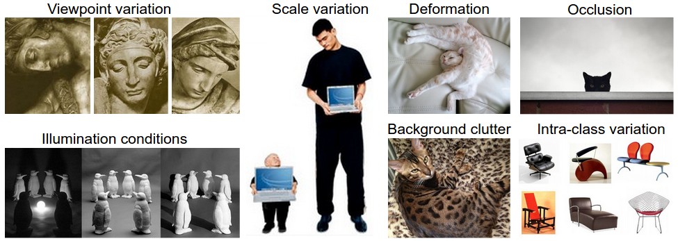
Challenges. Since this task of recognizing a visual concept (e.g. cat) is relatively trivial for a human to perform, it is worth considering the challenges involved from the perspective of a Computer Vision algorithm. As we present (an inexhaustive) list of challenges below, keep in mind the raw representation of images as a 3-D array of brightness values:

어려움(Challenges). 고양이 같은 시각적 개념을 알아보는 일은 사람에게는 별것 아니므로, 컴퓨터 비전 알고리즘의 입장에서 이 과제가 왜 어려운지 짚어볼 만하다. 아래에 어려움을 (전부는 아니지만) 나열하는데, 이미지가 밝기 값으로 이루어진 3차원 배열로 표현된다는 사실을 염두에 두고 읽자.

• Viewpoint variation. A single instance of an object can be oriented in many ways with respect to the camera.
• Scale variation. Visual classes often exhibit variation in their size (size in the real world, not only in terms of their extent in the image).
• Deformation. Many objects of interest are not rigid bodies and can be deformed in extreme ways.
• Occlusion. The objects of interest can be occluded. Sometimes only a small portion of an object (as little as few pixels) could be visible.
• Illumination conditions. The effects of illumination are drastic on the pixel level.
• Background clutter. The objects of interest may blend into their environment, making them hard to identify.
• Intra-class variation. The classes of interest can often be relatively broad, such as chair. There are many different types of these objects, each with their own appearance.

• 시점 변화(viewpoint variation). 같은 물체 하나도 카메라를 기준으로 여러 방향으로 놓일 수 있다.
• 크기 변화(scale variation). 시각적 클래스는 크기가 제각각인 경우가 많다. 이미지에서 차지하는 넓이만이 아니라 실제 세계에서의 크기도 그렇다.
• 변형(deformation). 관심 대상 상당수는 강체가 아니어서 형태가 극단적으로 바뀔 수 있다.
• 가려짐(occlusion). 관심 대상이 가려질 수 있다. 때로는 물체의 아주 일부만, 픽셀 몇 개에 불과할 만큼만 보이기도 한다.
• 조명 조건(illumination conditions). 조명이 픽셀 값에 미치는 영향은 대단히 크다.
• 배경 혼입(background clutter). 관심 대상이 주변 환경에 묻혀 알아보기 어려울 수 있다.
• 클래스 내 변화(intra-class variation). 관심 클래스는 의자처럼 범위가 넓은 경우가 많다. 그 안에는 저마다 생김새가 다른 여러 종류가 들어 있다.

A good image classification model must be invariant to the cross product of all these variations, while simultaneously retaining sensitivity to the inter-class variations.

좋은 이미지 분류 모델은 이 모든 변화의 조합에 대해 불변이면서, 동시에 클래스 사이의 차이에는 민감해야 한다.

Data-driven approach. How might we go about writing an algorithm that can classify images into distinct categories? Unlike writing an algorithm for, for example, sorting a list of numbers, it is not obvious how one might write an algorithm for identifying cats in images. Therefore, instead of trying to specify what every one of the categories of interest look like directly in code, the approach that we will take is not unlike one you would take with a child: we’re going to provide the computer with many examples of each class and then develop learning algorithms that look at these examples and learn about the visual appearance of each class. This approach is referred to as a data-driven approach, since it relies on first accumulating a training dataset of labeled images. Here is an example of what such a dataset might look like:

데이터 기반 접근법(data-driven approach). 이미지를 서로 다른 카테고리로 분류하는 알고리즘은 어떻게 짜야 할까? 숫자 목록을 정렬하는 알고리즘과 달리, 이미지에서 고양이를 찾아내는 알고리즘을 어떻게 짤지는 전혀 자명하지 않다. 그래서 관심 있는 카테고리 하나하나가 어떻게 생겼는지를 코드로 직접 명시하는 대신, 아이를 가르칠 때와 크게 다르지 않은 방식을 택한다. 각 클래스의 예시를 컴퓨터에 잔뜩 보여주고, 그 예시들을 살펴 각 클래스의 시각적 생김새를 배우는 학습 알고리즘을 만드는 것이다. 이 방식은 레이블이 붙은 이미지로 이루어진 학습 데이터셋(training dataset)을 먼저 모으는 데서 출발하므로 데이터 기반 접근법이라고 부른다. 그런 데이터셋의 예는 다음과 같다.

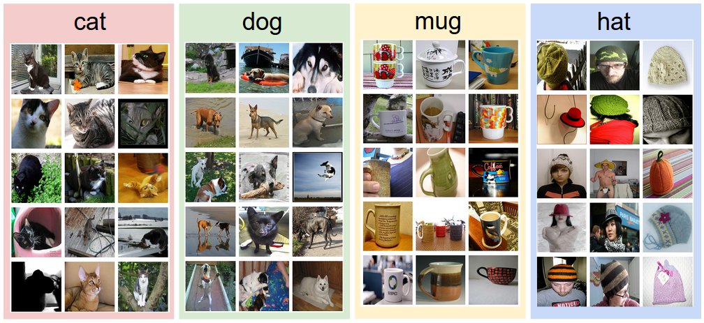An example training set for four visual categories. In practice we may have thousands of categories and hundreds of thousands of images for each category.

네 개 시각 카테고리에 대한 학습 집합 예시. 실제로는 카테고리가 수천 개이고 카테고리마다 이미지가 수십만 장일 수 있다.

The image classification pipeline. We’ve seen that the task in Image Classification is to take an array of pixels that represents a single image and assign a label to it. Our complete pipeline can be formalized as follows:

이미지 분류 파이프라인. 이미지 분류의 과제가 이미지 한 장을 나타내는 픽셀 배열을 받아 거기에 레이블을 붙이는 것임을 보았다. 전체 파이프라인은 다음과 같이 정리할 수 있다.

• Input: Our input consists of a set of N images, each labeled with one of K different classes. We refer to this data as the training set.
• Learning: Our task is to use the training set to learn what every one of the classes looks like. We refer to this step as training a classifier, or learning a model.
• Evaluation: In the end, we evaluate the quality of the classifier by asking it to predict labels for a new set of images that it has never seen before. We will then compare the true labels of these images to the ones predicted by the classifier. Intuitively, we’re hoping that a lot of the predictions match up with the true answers (which we call the ground truth).

• 입력: N장의 이미지로 이루어진 집합을 입력으로 받는다. 각 이미지에는 서로 다른 K개 클래스 중 하나가 레이블로 붙어 있다. 이 데이터를 학습 집합(training set)이라고 부른다.
• 학습: 학습 집합을 이용해 각 클래스가 어떻게 생겼는지 배우는 것이 우리의 과제다. 이 단계를 분류기 학습 또는 모델 학습이라고 부른다.
• 평가: 마지막으로 분류기가 한 번도 본 적 없는 새 이미지 집합의 레이블을 예측하게 해서 분류기의 품질을 평가한다. 그런 다음 이 이미지들의 실제 레이블과 분류기가 예측한 레이블을 비교한다. 직관적으로는 예측 상당수가 정답(ground truth라고 부른다)과 맞아떨어지기를 기대한다.

Nearest Neighbor Classifier

As our first approach, we will develop what we call a Nearest Neighbor Classifier. This classifier has nothing to do with Convolutional Neural Networks and it is very rarely used in practice, but it will allow us to get an idea about the basic approach to an image classification problem.

첫 접근으로 최근접 이웃 분류기(nearest neighbor classifier)라고 부르는 것을 만들어본다. 이 분류기는 합성곱 신경망과는 아무 관련이 없고 실제로 쓰이는 일도 거의 없지만, 이미지 분류 문제에 접근하는 기본 방식을 감 잡는 데는 도움이 된다.

Example image classification dataset: CIFAR-10. One popular toy image classification dataset is the CIFAR-10 dataset. This dataset consists of 60,000 tiny images that are 32 pixels high and wide. Each image is labeled with one of 10 classes (for example “airplane, automobile, bird, etc”). These 60,000 images are partitioned into a training set of 50,000 images and a test set of 10,000 images. In the image below you can see 10 random example images from each one of the 10 classes:

이미지 분류 데이터셋 예시: CIFAR-10. 널리 쓰이는 장난감 이미지 분류 데이터셋으로 CIFAR-10 데이터셋이 있다. 이 데이터셋은 가로세로 32픽셀짜리 작은 이미지 60,000장으로 이루어진다. 각 이미지에는 10개 클래스 중 하나가 레이블로 붙어 있다(예: “airplane, automobile, bird 등”). 이 60,000장은 학습 집합 50,000장과 테스트 집합 10,000장으로 나뉜다. 아래 그림에서 10개 클래스마다 무작위로 고른 예시 이미지 10장씩을 볼 수 있다.

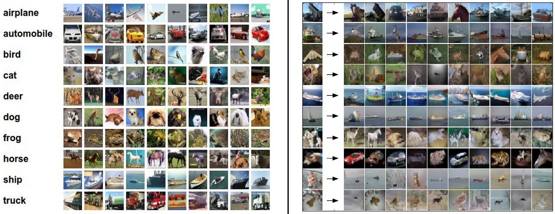Left: Example images from the CIFAR-10 dataset. Right: first column shows a few test images and next to each we show the top 10 nearest neighbors in the training set according to pixel-wise difference.

왼쪽: CIFAR-10 데이터셋의 예시 이미지. 오른쪽: 첫 열은 테스트 이미지 몇 장이고, 그 옆에는 픽셀 단위 차이를 기준으로 학습 집합에서 가장 가까운 이웃 10장을 나란히 놓았다.

Suppose now that we are given the CIFAR-10 training set of 50,000 images (5,000 images for every one of the labels), and we wish to label the remaining 10,000. The nearest neighbor classifier will take a test image, compare it to every single one of the training images, and predict the label of the closest training image. In the image above and on the right you can see an example result of such a procedure for 10 example test images. Notice that in only about 3 out of 10 examples an image of the same class is retrieved, while in the other 7 examples this is not the case. For example, in the 8th row the nearest training image to the horse head is a red car, presumably due to the strong black background. As a result, this image of a horse would in this case be mislabeled as a car.

이제 CIFAR-10 학습 집합 50,000장(레이블마다 5,000장)이 주어졌고 나머지 10,000장에 레이블을 붙이려 한다고 하자. 최근접 이웃 분류기는 테스트 이미지 한 장을 받아 학습 이미지 전부와 일일이 비교한 뒤, 가장 가까운 학습 이미지의 레이블을 답으로 내놓는다. 위 그림 오른쪽이 테스트 이미지 10장에 대해 이 절차를 돌린 결과다. 10개 중 3개 정도만 같은 클래스의 이미지가 찾아졌고 나머지 7개는 그렇지 않다는 점에 주목하자. 예를 들어 여덟 번째 행에서는 말 머리에 가장 가까운 학습 이미지가 빨간 자동차인데, 검은 배경이 강하게 작용한 탓으로 보인다. 그 결과 이 말 이미지는 자동차로 잘못 분류된다.

You may have noticed that we left unspecified the details of exactly how we compare two images, which in this case are just two blocks of 32 x 32 x 3. One of the simplest possibilities is to compare the images pixel by pixel and add up all the differences. In other words, given two images and representing them as vectors \(I_1, I_2\) , a reasonable choice for comparing them might be the L1 distance:

\[d_1 (I_1, I_2) = \sum_{p} \left| I^p_1 - I^p_2 \right|\]

두 이미지를 정확히 어떻게 비교하는지는 아직 정하지 않았다는 것을 눈치챘을 것이다. 여기서 두 이미지는 32 x 32 x 3짜리 숫자 덩어리 두 개일 뿐이다. 가장 단순한 방법 중 하나는 픽셀 하나하나를 비교해 차이를 모두 더하는 것이다. 다시 말해 두 이미지를 벡터 \(I_1, I_2\)로 볼 때, 둘을 비교하는 합리적인 선택 하나는 L1 거리(L1 distance)다.

역주. \(I^p_1\)의 위첨자 \(p\)는 거듭제곱이 아니라 픽셀의 번호다. 즉 \(I^p_1\)은 첫 번째 이미지의 \(p\)번째 픽셀 값이고, \(\sum_p\)는 이미지의 모든 픽셀을 훑는다는 뜻이다. CIFAR-10 이미지라면 \(p\)는 1부터 3,072(= 32 x 32 x 3)까지 돈다.

Where the sum is taken over all pixels. Here is the procedure visualized:

여기서 합은 모든 픽셀에 대해 취한다. 이 절차를 그림으로 보면 다음과 같다.

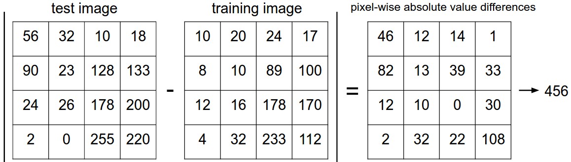An example of using pixel-wise differences to compare two images with L1 distance (for one color channel in this example). Two images are subtracted elementwise and then all differences are added up to a single number. If two images are identical the result will be zero. But if the images are very different the result will be large.

L1 거리로 두 이미지를 비교할 때 픽셀 단위 차이를 쓰는 예. 이 예시에서는 색 채널 하나만 보였다. 두 이미지를 원소별로 빼고 그 차이를 모두 더해 숫자 하나로 만든다. 두 이미지가 같으면 결과는 0이 되고, 많이 다르면 결과가 커진다.

Let’s also look at how we might implement the classifier in code. First, let’s load the CIFAR-10 data into memory as 4 arrays: the training data/labels and the test data/labels. In the code below, Xtr (of size 50,000 x 32 x 32 x 3) holds all the images in the training set, and a corresponding 1-dimensional array Ytr (of length 50,000) holds the training labels (from 0 to 9):

이 분류기를 코드로 어떻게 구현하는지도 살펴보자. 먼저 CIFAR-10 데이터를 학습 데이터/레이블과 테스트 데이터/레이블, 네 개 배열로 메모리에 올린다. 아래 코드에서 Xtr(크기 50,000 x 32 x 32 x 3)는 학습 집합의 모든 이미지를 담고, 이에 대응하는 1차원 배열 Ytr(길이 50,000)는 0부터 9까지의 학습 레이블을 담는다.

Xtr, Ytr, Xte, Yte = load_CIFAR10('data/cifar10/') # a magic function we provide
# flatten out all images to be one-dimensional
Xtr_rows = Xtr.reshape(Xtr.shape[0], 32 * 32 * 3) # Xtr_rows becomes 50000 x 3072
Xte_rows = Xte.reshape(Xte.shape[0], 32 * 32 * 3) # Xte_rows becomes 10000 x 3072

Now that we have all images stretched out as rows, here is how we could train and evaluate a classifier:

모든 이미지를 행 벡터로 펼쳤으니, 이제 분류기를 학습시키고 평가하는 방법은 다음과 같다.

nn = NearestNeighbor() # create a Nearest Neighbor classifier class
nn.train(Xtr_rows, Ytr) # train the classifier on the training images and labels
Yte_predict = nn.predict(Xte_rows) # predict labels on the test images
# and now print the classification accuracy, which is the average number
# of examples that are correctly predicted (i.e. label matches)
print 'accuracy: %f' % ( np.mean(Yte_predict == Yte) )

Notice that as an evaluation criterion, it is common to use the accuracy, which measures the fraction of predictions that were correct. Notice that all classifiers we will build satisfy this one common API: they have a train(X,y) function that takes the data and the labels to learn from. Internally, the class should build some kind of model of the labels and how they can be predicted from the data. And then there is a predict(X) function, which takes new data and predicts the labels. Of course, we’ve left out the meat of things - the actual classifier itself. Here is an implementation of a simple Nearest Neighbor classifier with the L1 distance that satisfies this template:

평가 기준으로는 예측이 맞은 비율을 재는 정확도(accuracy)를 흔히 쓴다. 앞으로 만들 분류기가 모두 같은 API 하나를 따른다는 점에도 주목하자. 학습할 데이터와 레이블을 받는 train(X,y) 함수가 있고, 클래스 내부에서는 레이블이 데이터로부터 어떻게 예측되는지에 관한 모델을 어떤 형태로든 만들어둔다. 그리고 새 데이터를 받아 레이블을 예측하는 predict(X) 함수가 있다. 물론 정작 알맹이인 분류기 자체는 아직 비워두었다. 아래는 이 틀을 따르는, L1 거리를 쓰는 단순한 최근접 이웃 분류기의 구현이다.

역주. 이 강의 노트의 코드는 파이썬 2 기준이라 print 'accuracy: %f' % (...)처럼 print를 문(statement)으로 쓴다. 파이썬 3에서는 print('accuracy: %f' % (...))로 괄호를 씌워야 한다. load_CIFAR10은 표준 라이브러리 함수가 아니라 강의 과제 코드에 딸려 오는 데이터 적재 함수다. 코드는 원문과의 대조를 위해 손대지 않고 그대로 실었다.

import numpy as np

class NearestNeighbor(object):
  def __init__(self):
    pass

  def train(self, X, y):
    """ X is N x D where each row is an example. Y is 1-dimension of size N """
    # the nearest neighbor classifier simply remembers all the training data
    self.Xtr = X
    self.ytr = y

  def predict(self, X):
    """ X is N x D where each row is an example we wish to predict label for """
    num_test = X.shape[0]
    # lets make sure that the output type matches the input type
    Ypred = np.zeros(num_test, dtype = self.ytr.dtype)

    # loop over all test rows
    for i in range(num_test):
      # find the nearest training image to the i'th test image
      # using the L1 distance (sum of absolute value differences)
      distances = np.sum(np.abs(self.Xtr - X[i,:]), axis = 1)
      min_index = np.argmin(distances) # get the index with smallest distance
      Ypred[i] = self.ytr[min_index] # predict the label of the nearest example

    return Ypred

If you ran this code, you would see that this classifier only achieves 38.6% on CIFAR-10. That’s more impressive than guessing at random (which would give 10% accuracy since there are 10 classes), but nowhere near human performance (which is estimated at about 94%) or near state-of-the-art Convolutional Neural Networks that achieve about 95%, matching human accuracy (see the leaderboard of a recent Kaggle competition on CIFAR-10).

이 코드를 돌려보면 이 분류기가 CIFAR-10에서 38.6%밖에 얻지 못한다는 것을 알 수 있다. 클래스가 10개이므로 10%가 나오는 무작위 추측보다는 나은 결과지만, 사람의 성능(약 94%로 추정된다)이나 사람과 맞먹는 95% 근처를 달성하는 최신 합성곱 신경망에는 한참 못 미친다. CIFAR-10을 다룬 최근 Kaggle 대회의 리더보드를 참고하라.

The choice of distance. There are many other ways of computing distances between vectors. Another common choice could be to instead use the L2 distance, which has the geometric interpretation of computing the euclidean distance between two vectors. The distance takes the form:

\[d_2 (I_1, I_2) = \sqrt{\sum_{p} \left( I^p_1 - I^p_2 \right)^2}\]

거리의 선택. 벡터 사이의 거리를 계산하는 방법은 이 밖에도 많다. 또 하나 흔한 선택은 L2 거리(L2 distance)인데, 두 벡터 사이의 유클리드 거리를 계산한다는 기하학적 해석을 갖는다. 이 거리는 다음과 같은 형태다.

In other words we would be computing the pixelwise difference as before, but this time we square all of them, add them up and finally take the square root. In numpy, using the code from above we would need to only replace a single line of code. The line that computes the distances:

다시 말해 앞에서처럼 픽셀 단위 차이를 구하되, 이번에는 그 차이를 모두 제곱해 더한 뒤 마지막에 제곱근을 취한다. numpy에서는 위 코드에서 딱 한 줄만 바꾸면 된다. 거리를 계산하는 줄이다.

distances = np.sqrt(np.sum(np.square(self.Xtr - X[i,:]), axis = 1))

Note that I included the np.sqrt call above, but in a practical nearest neighbor application we could leave out the square root operation because square root is a monotonic function. That is, it scales the absolute sizes of the distances but it preserves the ordering, so the nearest neighbors with or without it are identical. If you ran the Nearest Neighbor classifier on CIFAR-10 with this distance, you would obtain 35.4% accuracy (slightly lower than our L1 distance result).

위에서 np.sqrt 호출을 넣어두긴 했지만, 실제 최근접 이웃 응용에서는 제곱근을 생략해도 된다. 제곱근이 단조 함수(monotonic function)이기 때문이다. 즉 거리의 절대적인 크기는 바꾸지만 순서는 그대로 보존하므로, 제곱근을 취하든 말든 최근접 이웃은 똑같다. CIFAR-10에서 이 거리로 최근접 이웃 분류기를 돌리면 35.4%의 정확도가 나온다. L1 거리 결과보다 조금 낮다.

L1 vs. L2. It is interesting to consider differences between the two metrics. In particular, the L2 distance is much more unforgiving than the L1 distance when it comes to differences between two vectors. That is, the L2 distance prefers many medium disagreements to one big one. L1 and L2 distances (or equivalently the L1/L2 norms of the differences between a pair of images) are the most commonly used special cases of a p-norm.

L1 대 L2. 두 척도의 차이를 짚어볼 만하다. 특히 L2 거리는 두 벡터의 차이를 다룰 때 L1 거리보다 훨씬 가혹하다. 즉 L2 거리는 한 곳에서 크게 어긋나느니 여러 곳에서 적당히 어긋나는 쪽을 선호한다. L1 거리와 L2 거리, 달리 말해 두 이미지 차이의 L1/L2 노름은 p-노름의 특수한 경우 가운데 가장 널리 쓰이는 둘이다.

보충: L1과 L2가 어긋남을 다루는 방식

“한 번 크게 어긋나느니 여러 번 적당히 어긋나는 쪽을 선호한다”는 말은 숫자로 보면 분명해진다. 어긋난 총량이 같은 두 차이 벡터를 놓고 L1과 L2를 각각 재보자.

import numpy as np

# 두 이미지의 픽셀 단위 차이. 어긋난 총량(L1)은 같지만 퍼진 정도가 다르다.
spread = np.array([25, 25, 25, 25])       # 네 픽셀에서 조금씩 어긋남
concentrated = np.array([100, 0, 0, 0])   # 한 픽셀에서 크게 어긋남

for name, d in [("spread", spread), ("concentrated", concentrated)]:
    l1 = np.sum(np.abs(d))
    l2 = np.sqrt(np.sum(np.square(d)))
    print(f"{name:<13} L1 = {l1:5.1f}   L2 = {l2:5.1f}")

spread        L1 = 100.0   L2 =  50.0
concentrated  L1 = 100.0   L2 = 100.0

L1은 둘을 구분하지 못하고 똑같이 100으로 본다. 반면 L2는 어긋남이 한곳에 몰린 쪽을 두 배 더 멀다고 판단한다. 제곱이 큰 값을 훨씬 크게 부풀리기 때문이다. 이미지로 옮기면, L2를 쓰는 분류기는 전체적으로 조금씩 흐릿하게 다른 이미지보다 한 부분이 확 다른 이미지를 더 멀리 있다고 본다.

k - Nearest Neighbor Classifier

You may have noticed that it is strange to only use the label of the nearest image when we wish to make a prediction. Indeed, it is almost always the case that one can do better by using what’s called a k-Nearest Neighbor Classifier. The idea is very simple: instead of finding the single closest image in the training set, we will find the top k closest images, and have them vote on the label of the test image. In particular, when k = 1, we recover the Nearest Neighbor classifier. Intuitively, higher values of k have a smoothing effect that makes the classifier more resistant to outliers:

예측을 할 때 가장 가까운 이미지 한 장의 레이블만 쓰는 것이 이상하다고 느꼈을 수 있다. 실제로 k-최근접 이웃 분류기(k-Nearest Neighbor Classifier)라고 부르는 것을 쓰면 거의 언제나 더 나은 결과를 얻는다. 발상은 아주 단순하다. 학습 집합에서 가장 가까운 이미지 한 장만 찾는 대신 가장 가까운 k장을 찾아, 이들이 테스트 이미지의 레이블을 투표로 정하게 한다. 특히 k = 1이면 최근접 이웃 분류기가 된다. 직관적으로 k가 커질수록 평활화 효과가 생겨 분류기가 이상치에 덜 흔들린다.

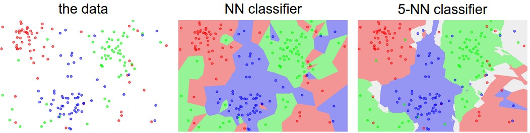An example of the difference between Nearest Neighbor and a 5-Nearest Neighbor classifier, using 2-dimensional points and 3 classes (red, blue, green). The colored regions show the decision boundaries induced by the classifier with an L2 distance. The white regions show points that are ambiguously classified (i.e. class votes are tied for at least two classes). Notice that in the case of a NN classifier, outlier datapoints (e.g. green point in the middle of a cloud of blue points) create small islands of likely incorrect predictions, while the 5-NN classifier smooths over these irregularities, likely leading to better generalization on the test data (not shown). Also note that the gray regions in the 5-NN image are caused by ties in the votes among the nearest neighbors (e.g. 2 neighbors are red, next two neighbors are blue, last neighbor is green).

최근접 이웃 분류기와 5-최근접 이웃 분류기의 차이를 2차원 점과 세 개 클래스(빨강, 파랑, 초록)로 보인 예. 색칠된 영역은 L2 거리를 쓰는 분류기가 만들어낸 결정 경계(decision boundary)다. 흰 영역은 분류가 모호한 점들, 즉 적어도 두 클래스의 득표가 같은 점들이다. NN 분류기에서는 이상치 데이터(예: 파란 점 무리 한가운데의 초록 점)가 잘못된 예측을 낳는 작은 섬을 만드는 반면, 5-NN 분류기는 이런 불규칙성을 매끄럽게 눌러 테스트 데이터에 대한 일반화(generalization)가 더 나아질 가능성이 크다(그림에는 나타나 있지 않다). 또한 5-NN 그림의 회색 영역은 최근접 이웃들의 득표가 동점이라 생긴 것이다(예: 이웃 2개가 빨강, 다음 2개가 파랑, 마지막 1개가 초록인 경우).

In practice, you will almost always want to use k-Nearest Neighbor. But what value of k should you use? We turn to this problem next.

실제로는 거의 언제나 k-최근접 이웃을 쓰고 싶을 것이다. 그런데 k는 어떤 값을 써야 할까? 이 문제를 다음에서 다룬다.

Validation sets for Hyperparameter tuning

The k-nearest neighbor classifier requires a setting for k. But what number works best? Additionally, we saw that there are many different distance functions we could have used: L1 norm, L2 norm, there are many other choices we didn’t even consider (e.g. dot products). These choices are called hyperparameters and they come up very often in the design of many Machine Learning algorithms that learn from data. It’s often not obvious what values/settings one should choose.

k-최근접 이웃 분류기는 k를 정해줘야 한다. 그런데 어떤 값이 가장 좋을까? 게다가 쓸 수 있는 거리 함수도 L1 노름, L2 노름 등 여러 가지였고, 아예 고려조차 하지 않은 선택지(예: 내적)도 많다. 이런 선택지를 하이퍼파라미터(hyperparameter)라고 부르며, 데이터로부터 학습하는 여러 머신러닝 알고리즘을 설계할 때 아주 자주 등장한다. 어떤 값이나 설정을 골라야 할지는 대개 자명하지 않다.

You might be tempted to suggest that we should try out many different values and see what works best. That is a fine idea and that’s indeed what we will do, but this must be done very carefully. In particular, we cannot use the test set for the purpose of tweaking hyperparameters. Whenever you’re designing Machine Learning algorithms, you should think of the test set as a very precious resource that should ideally never be touched until one time at the very end. Otherwise, the very real danger is that you may tune your hyperparameters to work well on the test set, but if you were to deploy your model you could see a significantly reduced performance. In practice, we would say that you overfit to the test set. Another way of looking at it is that if you tune your hyperparameters on the test set, you are effectively using the test set as the training set, and therefore the performance you achieve on it will be too optimistic with respect to what you might actually observe when you deploy your model. But if you only use the test set once at end, it remains a good proxy for measuring the generalization of your classifier (we will see much more discussion surrounding generalization later in the class).

여러 값을 시도해보고 가장 잘 되는 것을 고르면 되지 않느냐고 할 수 있다. 좋은 생각이고 실제로도 그렇게 할 것이지만, 아주 조심스럽게 해야 한다. 특히 하이퍼파라미터를 조정하는 데 테스트 집합을 써서는 안 된다. 머신러닝 알고리즘을 설계할 때 테스트 집합은 대단히 귀한 자원이라고 생각해야 하며, 맨 마지막에 딱 한 번 쓰기 전까지는 손대지 않는 것이 이상적이다. 그러지 않으면 테스트 집합에서만 잘 동작하도록 하이퍼파라미터를 맞추게 되고, 모델을 실제로 배포했을 때 성능이 눈에 띄게 떨어지는 아주 현실적인 위험이 생긴다. 이런 상황을 두고 테스트 집합에 과적합(overfitting)했다고 말한다. 달리 보면, 테스트 집합에서 하이퍼파라미터를 조정하는 것은 사실상 테스트 집합을 학습 집합으로 쓰는 셈이고, 따라서 거기서 얻은 성능은 실제로 배포했을 때 관찰될 성능에 비해 지나치게 낙관적이다. 반면 테스트 집합을 맨 마지막에 한 번만 쓴다면, 그것은 분류기의 일반화 성능을 재는 좋은 대리 지표로 남는다. 일반화에 관해서는 수업 뒤쪽에서 훨씬 자세히 논의한다.

Evaluate on the test set only a single time, at the very end.

테스트 집합에서의 평가는 맨 마지막에 딱 한 번만 한다.

Luckily, there is a correct way of tuning the hyperparameters and it does not touch the test set at all. The idea is to split our training set in two: a slightly smaller training set, and what we call a validation set. Using CIFAR-10 as an example, we could for example use 49,000 of the training images for training, and leave 1,000 aside for validation. This validation set is essentially used as a fake test set to tune the hyper-parameters.

다행히 하이퍼파라미터를 조정하는 올바른 방법이 있고, 그 방법은 테스트 집합에 전혀 손대지 않는다. 발상은 학습 집합을 둘로 쪼개는 것이다. 조금 작아진 학습 집합과, 검증 집합(validation set)이라고 부르는 것으로 나눈다. CIFAR-10을 예로 들면 학습 이미지 중 49,000장을 학습에 쓰고 1,000장을 검증용으로 떼어둘 수 있다. 이 검증 집합은 하이퍼파라미터를 조정하기 위한 가짜 테스트 집합 역할을 한다.

Here is what this might look like in the case of CIFAR-10:

CIFAR-10의 경우 코드로는 다음과 같은 모습이 된다.

# assume we have Xtr_rows, Ytr, Xte_rows, Yte as before
# recall Xtr_rows is 50,000 x 3072 matrix
Xval_rows = Xtr_rows[:1000, :] # take first 1000 for validation
Yval = Ytr[:1000]
Xtr_rows = Xtr_rows[1000:, :] # keep last 49,000 for train
Ytr = Ytr[1000:]

# find hyperparameters that work best on the validation set
validation_accuracies = []
for k in [1, 3, 5, 10, 20, 50, 100]:

  # use a particular value of k and evaluation on validation data
  nn = NearestNeighbor()
  nn.train(Xtr_rows, Ytr)
  # here we assume a modified NearestNeighbor class that can take a k as input
  Yval_predict = nn.predict(Xval_rows, k = k)
  acc = np.mean(Yval_predict == Yval)
  print 'accuracy: %f' % (acc,)

  # keep track of what works on the validation set
  validation_accuracies.append((k, acc))

By the end of this procedure, we could plot a graph that shows which values of k work best. We would then stick with this value and evaluate once on the actual test set.

이 절차가 끝나면 어떤 k 값이 가장 좋은지 보여주는 그래프를 그릴 수 있다. 그다음 그 값으로 확정하고 실제 테스트 집합에서 딱 한 번 평가한다.

Split your training set into training set and a validation set. Use validation set to tune all hyperparameters. At the end run a single time on the test set and report performance.

학습 집합을 학습 집합과 검증 집합으로 나눈다. 모든 하이퍼파라미터는 검증 집합으로 조정한다. 마지막에 테스트 집합에서 한 번만 돌리고 그 성능을 보고한다.

Cross-validation. In cases where the size of your training data (and therefore also the validation data) might be small, people sometimes use a more sophisticated technique for hyperparameter tuning called cross-validation. Working with our previous example, the idea is that instead of arbitrarily picking the first 1000 datapoints to be the validation set and rest training set, you can get a better and less noisy estimate of how well a certain value of k works by iterating over different validation sets and averaging the performance across these. For example, in 5-fold cross-validation, we would split the training data into 5 equal folds, use 4 of them for training, and 1 for validation. We would then iterate over which fold is the validation fold, evaluate the performance, and finally average the performance across the different folds.

교차 검증(cross-validation). 학습 데이터의 크기가 작아 검증 데이터도 작아지는 경우에는, 하이퍼파라미터 조정에 교차 검증이라는 좀 더 정교한 기법을 쓰기도 한다. 앞의 예로 말하면, 앞쪽 1,000개를 임의로 검증 집합으로 삼고 나머지를 학습 집합으로 삼는 대신, 검증 집합을 바꿔가며 여러 번 돌리고 그 성능을 평균 내는 것이다. 그러면 특정 k 값이 얼마나 잘 동작하는지를 잡음이 덜한 방식으로 더 잘 추정할 수 있다. 예를 들어 5-겹 교차 검증에서는 학습 데이터를 같은 크기의 5개 겹으로 나눠 4개를 학습에, 1개를 검증에 쓴다. 그다음 어느 겹이 검증 겹이 되는지를 바꿔가며 반복해 성능을 측정하고, 마지막에 겹들의 성능을 평균 낸다.

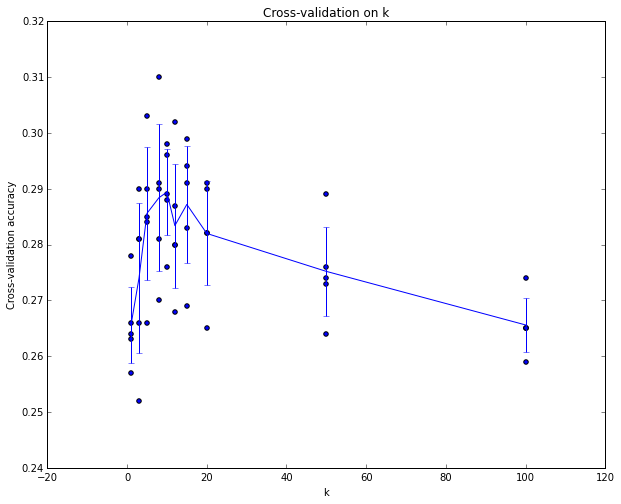Example of a 5-fold cross-validation run for the parameter k. For each value of k we train on 4 folds and evaluate on the 5th. Hence, for each k we receive 5 accuracies on the validation fold (accuracy is the y-axis, each result is a point). The trend line is drawn through the average of the results for each k and the error bars indicate the standard deviation. Note that in this particular case, the cross-validation suggests that a value of about k = 7 works best on this particular dataset (corresponding to the peak in the plot). If we used more than 5 folds, we might expect to see a smoother (i.e. less noisy) curve.

파라미터 k에 대한 5-겹 교차 검증 실행 예. 각 k 값마다 4개 겹으로 학습하고 5번째 겹에서 평가한다. 따라서 k마다 검증 겹에서 정확도를 5개 얻는다(y축이 정확도이고 결과 하나가 점 하나다). 추세선은 각 k의 결과 평균을 이은 것이고, 오차 막대는 표준편차를 나타낸다. 이 데이터셋에서는 교차 검증 결과 k = 7 근처가 가장 좋다고 나왔다. 그래프의 봉우리에 해당한다. 겹을 5개보다 많이 썼다면 더 매끄러운, 즉 잡음이 덜한 곡선을 볼 수 있었을 것이다.

In practice. In practice, people prefer to avoid cross-validation in favor of having a single validation split, since cross-validation can be computationally expensive. The splits people tend to use is between 50%-90% of the training data for training and rest for validation. However, this depends on multiple factors: For example if the number of hyperparameters is large you may prefer to use bigger validation splits. If the number of examples in the validation set is small (perhaps only a few hundred or so), it is safer to use cross-validation. Typical number of folds you can see in practice would be 3-fold, 5-fold or 10-fold cross-validation.

실무에서는. 실무에서는 교차 검증의 계산 비용이 크기 때문에 이를 피하고 검증 분할 하나만 두는 쪽을 선호한다. 흔히 학습 데이터의 50%~90%를 학습에, 나머지를 검증에 쓴다. 다만 이 비율은 여러 요인에 따라 달라진다. 예를 들어 하이퍼파라미터 개수가 많다면 검증 분할을 더 크게 잡는 편이 나을 수 있다. 검증 집합의 예시 수가 적다면(수백 개 정도에 불과하다면) 교차 검증을 쓰는 편이 안전하다. 실무에서 흔히 보이는 겹 수는 3-겹, 5-겹, 10-겹이다.

Common data splits. A training and test set is given. The training set is split into folds (for example 5 folds here). The folds 1-4 become the training set. One fold (e.g. fold 5 here in yellow) is denoted as the Validation fold and is used to tune the hyperparameters. Cross-validation goes a step further and iterates over the choice of which fold is the validation fold, separately from 1-5. This would be referred to as 5-fold cross-validation. In the very end once the model is trained and all the best hyperparameters were determined, the model is evaluated a single time on the test data (red).

흔히 쓰는 데이터 분할. 학습 집합과 테스트 집합이 주어진다. 학습 집합은 여러 겹으로 나뉜다(여기서는 5개 겹). 1~4번 겹이 학습 집합이 된다. 겹 하나(여기서는 노란색 5번 겹)를 검증 겹이라 부르고 하이퍼파라미터를 조정하는 데 쓴다. 교차 검증은 여기서 한발 더 나아가, 어느 겹을 검증 겹으로 삼을지를 1번부터 5번까지 바꿔가며 반복한다. 이를 5-겹 교차 검증이라고 부른다. 맨 마지막에 모델을 다 학습하고 최적 하이퍼파라미터를 모두 정한 뒤, 테스트 데이터(빨간색)에서 딱 한 번 평가한다.

Pros and Cons of Nearest Neighbor classifier.

최근접 이웃 분류기의 장단점.

It is worth considering some advantages and drawbacks of the Nearest Neighbor classifier. Clearly, one advantage is that it is very simple to implement and understand. Additionally, the classifier takes no time to train, since all that is required is to store and possibly index the training data. However, we pay that computational cost at test time, since classifying a test example requires a comparison to every single training example. This is backwards, since in practice we often care about the test time efficiency much more than the efficiency at training time. In fact, the deep neural networks we will develop later in this class shift this tradeoff to the other extreme: They are very expensive to train, but once the training is finished it is very cheap to classify a new test example. This mode of operation is much more desirable in practice.

최근접 이웃 분류기의 장점과 단점을 짚어볼 만하다. 우선 구현과 이해가 아주 쉽다는 것이 분명한 장점이다. 또한 학습 데이터를 저장하고 필요하면 색인만 만들면 되므로 학습에 시간이 전혀 들지 않는다. 그러나 그 계산 비용은 테스트 시점에 치른다. 테스트 예시 하나를 분류하려면 학습 예시 전부와 비교해야 하기 때문이다. 이는 앞뒤가 뒤바뀐 것인데, 실무에서는 학습 시점의 효율보다 테스트 시점의 효율이 훨씬 중요한 경우가 많기 때문이다. 실제로 이 수업 뒤쪽에서 만들 심층 신경망은 이 트레이드오프를 정반대 극단으로 옮긴다. 학습에는 비용이 아주 많이 들지만, 학습이 끝나고 나면 새 테스트 예시를 분류하는 비용은 아주 싸다. 실무에서는 이런 동작 방식이 훨씬 바람직하다.

As an aside, the computational complexity of the Nearest Neighbor classifier is an active area of research, and several Approximate Nearest Neighbor (ANN) algorithms and libraries exist that can accelerate the nearest neighbor lookup in a dataset (e.g. FLANN). These algorithms allow one to trade off the correctness of the nearest neighbor retrieval with its space/time complexity during retrieval, and usually rely on a pre-processing/indexing stage that involves building a kdtree, or running the k-means algorithm.

덧붙이면 최근접 이웃 분류기의 계산 복잡도는 지금도 활발히 연구되는 주제이며, 데이터셋에서 최근접 이웃을 찾는 속도를 높여주는 근사 최근접 이웃(Approximate Nearest Neighbor, ANN) 알고리즘과 라이브러리가 여럿 있다(예: FLANN). 이런 알고리즘은 최근접 이웃 검색의 정확성을 검색 시점의 공간, 시간 복잡도와 맞바꾸며, 대개 kd 트리를 만들거나 k-means 알고리즘을 돌리는 전처리, 색인 단계에 의존한다.

The Nearest Neighbor Classifier may sometimes be a good choice in some settings (especially if the data is low-dimensional), but it is rarely appropriate for use in practical image classification settings. One problem is that images are high-dimensional objects (i.e. they often contain many pixels), and distances over high-dimensional spaces can be very counter-intuitive. The image below illustrates the point that the pixel-based L2 similarities we developed above are very different from perceptual similarities:

최근접 이웃 분류기는 어떤 상황에서는, 특히 데이터의 차원이 낮을 때는 좋은 선택일 수 있다. 그러나 실제 이미지 분류 상황에 쓰기에는 적절하지 않은 경우가 대부분이다. 한 가지 문제는 이미지가 고차원 객체라는 점이다. 즉 픽셀이 아주 많다. 그리고 고차원 공간에서의 거리는 대단히 반직관적일 수 있다. 아래 그림은 앞에서 다룬 픽셀 기반 L2 유사도가 사람이 느끼는 유사도와 아주 다르다는 것을 보여준다.

역주. 고차원에서 거리가 반직관적이 되는 데는 이유가 있다. 차원이 늘어날수록 임의의 두 점 사이 거리가 모두 비슷한 값으로 몰리는 현상이 나타난다. 가장 가까운 이웃과 가장 먼 이웃의 거리 차이가 상대적으로 줄어들어, “가장 가깝다”는 판단이 점점 의미를 잃는다는 뜻이다. CIFAR-10 이미지 하나는 3,072차원 벡터이므로 이 문제에서 자유롭지 않다. 더 근본적인 문제는 그다음 문단이 짚는 대로, 픽셀 공간에서의 거리 자체가 사람이 느끼는 유사도를 반영하지 못한다는 점이다.

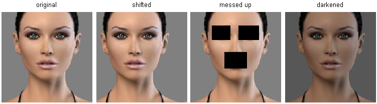Pixel-based distances on high-dimensional data (and images especially) can be very unintuitive. An original image (left) and three other images next to it that are all equally far away from it based on L2 pixel distance. Clearly, the pixel-wise distance does not correspond at all to perceptual or semantic similarity.

고차원 데이터, 특히 이미지에서 픽셀 기반 거리는 대단히 반직관적일 수 있다. 원본 이미지(왼쪽)와, L2 픽셀 거리 기준으로 원본에서 모두 똑같이 떨어져 있는 다른 이미지 세 장이다. 픽셀 단위 거리가 사람이 느끼는 유사도나 의미상의 유사도와 전혀 대응하지 않는다는 것이 분명하다.

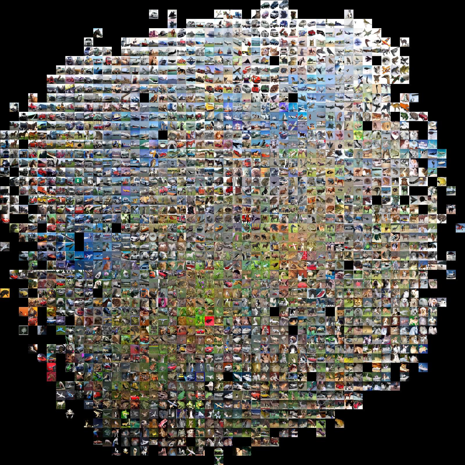
Here is one more visualization to convince you that using pixel differences to compare images is inadequate. We can use a visualization technique called t-SNE to take the CIFAR-10 images and embed them in two dimensions so that their (local) pairwise distances are best preserved. In this visualization, images that are shown nearby are considered to be very near according to the L2 pixelwise distance we developed above:

픽셀 차이로 이미지를 비교하는 것이 부적절하다는 점을 확실히 해줄 시각화를 하나 더 보자. t-SNE라는 시각화 기법을 쓰면 CIFAR-10 이미지를 (국소적인) 쌍별 거리가 최대한 보존되도록 2차원에 배치할 수 있다. 이 시각화에서 가까이 놓인 이미지들은 앞에서 다룬 L2 픽셀 거리 기준으로 아주 가깝다고 판단된 것들이다.

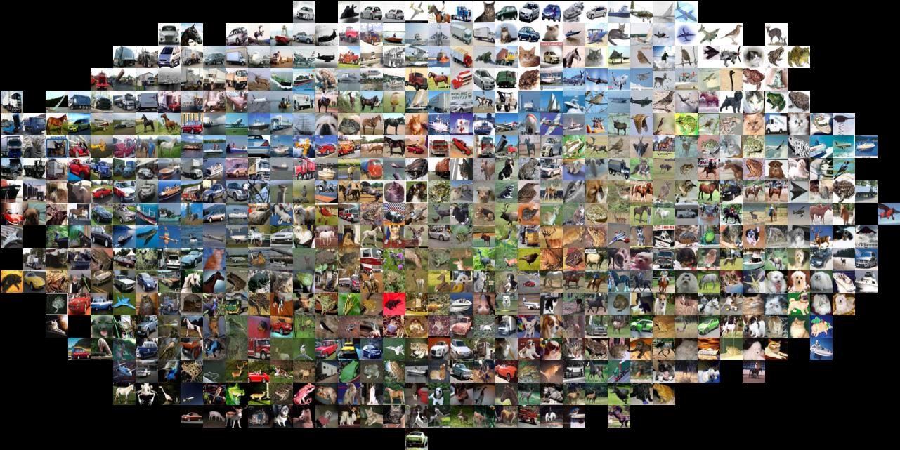CIFAR-10 images embedded in two dimensions with t-SNE. Images that are nearby on this image are considered to be close based on the L2 pixel distance. Notice the strong effect of background rather than semantic class differences. Click here for a bigger version of this visualization.

t-SNE로 2차원에 배치한 CIFAR-10 이미지. 이 그림에서 가까이 있는 이미지들은 L2 픽셀 거리 기준으로 가깝다고 판단된 것들이다. 의미상의 클래스 차이보다 배경이 훨씬 강하게 작용한다는 점에 주목하자. 더 큰 버전은 여기에서 볼 수 있다.

In particular, note that images that are nearby each other are much more a function of the general color distribution of the images, or the type of background rather than their semantic identity. For example, a dog can be seen very near a frog since both happen to be on white background. Ideally we would like images of all of the 10 classes to form their own clusters, so that images of the same class are nearby to each other regardless of irrelevant characteristics and variations (such as the background). However, to get this property we will have to go beyond raw pixels.

특히 서로 가까이 놓인 이미지들은 의미상의 정체보다 이미지 전체의 색 분포나 배경 종류에 훨씬 크게 좌우된다는 점에 주목하자. 예를 들어 개와 개구리가 아주 가까이 놓일 수 있는데, 둘 다 흰 배경 위에 있기 때문이다. 이상적으로는 10개 클래스가 각자의 군집을 이뤄서, 배경 같은 무관한 특성이나 변화와 상관없이 같은 클래스의 이미지끼리 가까이 놓이기를 바란다. 그러나 이 성질을 얻으려면 날 픽셀 값 너머로 나아가야 한다.

Summary

In summary:

정리하면 다음과 같다.

• We introduced the problem of Image Classification, in which we are given a set of images that are all labeled with a single category. We are then asked to predict these categories for a novel set of test images and measure the accuracy of the predictions.
• We introduced a simple classifier called the Nearest Neighbor classifier. We saw that there are multiple hyper-parameters (such as value of k, or the type of distance used to compare examples) that are associated with this classifier and that there was no obvious way of choosing them.
• We saw that the correct way to set these hyperparameters is to split your training data into two: a training set and a fake test set, which we call validation set. We try different hyperparameter values and keep the values that lead to the best performance on the validation set.
• If the lack of training data is a concern, we discussed a procedure called cross-validation, which can help reduce noise in estimating which hyperparameters work best.
• Once the best hyperparameters are found, we fix them and perform a single evaluation on the actual test set.
• We saw that Nearest Neighbor can get us about 40% accuracy on CIFAR-10. It is simple to implement but requires us to store the entire training set and it is expensive to evaluate on a test image.
• Finally, we saw that the use of L1 or L2 distances on raw pixel values is not adequate since the distances correlate more strongly with backgrounds and color distributions of images than with their semantic content.

• 이미지 분류 문제를 소개했다. 하나의 카테고리가 레이블로 붙은 이미지 집합이 주어지고, 새로운 테스트 이미지 집합에 대해 그 카테고리를 예측한 뒤 예측의 정확도를 재는 문제다.
• 최근접 이웃 분류기라는 단순한 분류기를 소개했다. 이 분류기에는 하이퍼파라미터가 여럿 딸려 있고(k 값이나 예시를 비교하는 데 쓰는 거리의 종류 등), 이를 고르는 자명한 방법은 없다는 것을 보았다.
• 이 하이퍼파라미터를 정하는 올바른 방법은 학습 데이터를 둘로 나누는 것임을 보았다. 학습 집합과, 검증 집합이라고 부르는 가짜 테스트 집합이다. 여러 하이퍼파라미터 값을 시도해보고 검증 집합에서 가장 좋은 성능을 내는 값을 택한다.
• 학습 데이터가 부족한 것이 걱정된다면 교차 검증이라는 절차를 쓸 수 있다. 어떤 하이퍼파라미터가 가장 좋은지 추정할 때 생기는 잡음을 줄여준다.
• 최적 하이퍼파라미터를 찾고 나면 그 값으로 고정하고 실제 테스트 집합에서 평가를 딱 한 번 수행한다.
• 최근접 이웃으로 CIFAR-10에서 40% 정도의 정확도를 얻을 수 있음을 보았다. 구현은 간단하지만 학습 집합 전체를 저장해야 하고 테스트 이미지 하나를 평가하는 비용이 크다.
• 마지막으로, 날 픽셀 값에 L1이나 L2 거리를 쓰는 것은 적절하지 않음을 보았다. 이 거리는 이미지의 의미 내용보다 배경과 색 분포에 훨씬 강하게 연동되기 때문이다.

In next lectures we will embark on addressing these challenges and eventually arrive at solutions that give 90% accuracies, allow us to completely discard the training set once learning is complete, and they will allow us to evaluate a test image in less than a millisecond.

다음 강의들에서는 이 어려움들을 하나씩 해결해 나가면서, 결국 90%대의 정확도를 내고, 학습이 끝나면 학습 집합을 통째로 버릴 수 있으며, 테스트 이미지 하나를 1밀리초도 안 되어 평가할 수 있는 해법에 이른다.

Summary: Applying kNN in practice

If you wish to apply kNN in practice (hopefully not on images, or perhaps as only a baseline) proceed as follows:

kNN을 실제로 적용하고 싶다면(이미지에는 쓰지 않기를 바라며, 쓴다면 기준선 정도로만) 다음 순서를 따른다.

1. Preprocess your data: Normalize the features in your data (e.g. one pixel in images) to have zero mean and unit variance. We will cover this in more detail in later sections, and chose not to cover data normalization in this section because pixels in images are usually homogeneous and do not exhibit widely different distributions, alleviating the need for data normalization.
2. If your data is very high-dimensional, consider using a dimensionality reduction technique such as PCA (wiki ref, CS229ref, blog ref), NCA (wiki ref, blog ref), or even Random Projections.
3. Split your training data randomly into train/val splits. As a rule of thumb, between 70-90% of your data usually goes to the train split. This setting depends on how many hyperparameters you have and how much of an influence you expect them to have. If there are many hyperparameters to estimate, you should err on the side of having larger validation set to estimate them effectively. If you are concerned about the size of your validation data, it is best to split the training data into folds and perform cross-validation. If you can afford the computational budget it is always safer to go with cross-validation (the more folds the better, but more expensive).
4. Train and evaluate the kNN classifier on the validation data (for all folds, if doing cross-validation) for many choices of k (e.g. the more the better) and across different distance types (L1 and L2 are good candidates)
5. If your kNN classifier is running too long, consider using an Approximate Nearest Neighbor library (e.g. FLANN) to accelerate the retrieval (at cost of some accuracy).
6. Take note of the hyperparameters that gave the best results. There is a question of whether you should use the full training set with the best hyperparameters, since the optimal hyperparameters might change if you were to fold the validation data into your training set (since the size of the data would be larger). In practice it is cleaner to not use the validation data in the final classifier and consider it to be burned on estimating the hyperparameters. Evaluate the best model on the test set. Report the test set accuracy and declare the result to be the performance of the kNN classifier on your data.

1. 데이터를 전처리한다. 데이터의 특성(예: 이미지의 픽셀 하나)을 평균 0, 분산 1이 되도록 정규화(normalization)한다. 이 내용은 뒤쪽 절에서 더 자세히 다룬다. 이미지의 픽셀은 대체로 성질이 균일하고 분포가 크게 다르지 않아 데이터 정규화의 필요가 덜하므로, 이 절에서는 다루지 않기로 했다.
2. 데이터의 차원이 아주 높다면 PCA(위키, CS229 자료, 블로그 글)나 NCA(위키, 블로그 글) 같은 차원 축소 기법, 혹은 랜덤 프로젝션을 쓰는 것을 고려한다.
3. 학습 데이터를 무작위로 학습/검증으로 나눈다. 경험칙으로는 데이터의 70~90%를 학습 쪽에 둔다. 이 비율은 하이퍼파라미터가 몇 개인지, 그리고 그것들이 얼마나 큰 영향을 미칠 것으로 보는지에 따라 달라진다. 추정할 하이퍼파라미터가 많다면 검증 집합을 크게 잡아 제대로 추정하는 쪽으로 기우는 편이 좋다. 검증 데이터의 크기가 걱정된다면 학습 데이터를 겹으로 나눠 교차 검증을 하는 것이 가장 낫다. 계산 예산을 감당할 수 있다면 언제나 교차 검증이 더 안전하다(겹이 많을수록 좋지만 그만큼 비싸다).
4. 검증 데이터에서(교차 검증을 한다면 모든 겹에 대해) 여러 k 값(예: 많을수록 좋다)과 여러 거리 종류(L1과 L2가 좋은 후보다)로 kNN 분류기를 학습하고 평가한다.
5. kNN 분류기가 너무 오래 걸린다면 근사 최근접 이웃 라이브러리(예: FLANN)로 검색 속도를 높이는 것을 고려한다. 정확도를 조금 내주는 대가다.
6. 가장 좋은 결과를 낸 하이퍼파라미터를 기록해둔다. 검증 데이터를 학습 집합에 합쳐 전체 학습 집합에 최적 하이퍼파라미터를 그대로 써야 하는지는 따져볼 문제다. 데이터 크기가 커지면 최적 하이퍼파라미터가 달라질 수 있기 때문이다. 실무에서는 최종 분류기에 검증 데이터를 쓰지 않고, 하이퍼파라미터 추정에 태워버린 것으로 치는 편이 깔끔하다. 가장 좋은 모델을 테스트 집합에서 평가한다. 테스트 집합 정확도를 보고하고, 그 값을 해당 데이터에 대한 kNN 분류기의 성능으로 선언한다.

Further Reading

Here are some (optional) links you may find interesting for further reading:

더 읽어보면 좋을 (선택) 링크들이다.

• A Few Useful Things to Know about Machine Learning, where especially section 6 is related but the whole paper is a warmly recommended reading.
• Recognizing and Learning Object Categories, a short course of object categorization at ICCV 2005.

• A Few Useful Things to Know about Machine Learning. 특히 6절이 이 내용과 관련이 깊지만, 논문 전체를 읽어볼 것을 권한다.
• Recognizing and Learning Object Categories. ICCV 2005에서 열린 물체 분류 단기 강좌다.