02. Linear Classification: Support Vector Machine, Softmax

원문: Linear Classification: Support Vector Machine, Softmax — CS231n: Convolutional Neural Networks for Visual Recognition (Stanford University) · © 2015 Andrej Karpathy, MIT License

원문을 문단 단위로 인용하고 그 아래에 한국어 번역을 붙였다. 인용 블록이 원문, 그 아래 문단이 번역이며, 역주 박스와 보충 섹션은 원문에 없는 추가 내용이다.

Table of Contents:

목차는 다음과 같다.

• Linear Classification
• Parameterized mapping from images to label scores
• Interpreting a linear classifier
• Loss function
• Multiclass Support Vector Machine loss
• Practical Considerations
• Softmax classifier
• SVM vs. Softmax
• Interactive web demo
• Summary
• Further Reading

• 선형 분류
• 이미지에서 클래스 점수로 가는 매개변수화된 매핑
• 선형 분류기 해석하기
• 손실 함수
• Multiclass Support Vector Machine 손실
• 실전에서 고려할 것들
• Softmax 분류기
• SVM 대 Softmax
• 대화형 웹 데모
• 정리
• 더 읽을거리

Linear Classification

In the last section we introduced the problem of Image Classification, which is the task of assigning a single label to an image from a fixed set of categories. Moreover, we described the k-Nearest Neighbor (kNN) classifier which labels images by comparing them to (annotated) images from the training set. As we saw, kNN has a number of disadvantages:

지난 절에서 고정된 카테고리 집합에서 레이블 하나를 골라 이미지에 붙이는 작업, 즉 이미지 분류 문제를 소개했다. 또한 학습 집합에 있는 (레이블이 달린) 이미지들과 비교해 이미지에 레이블을 매기는 k-최근접 이웃(kNN) 분류기도 살펴봤다. 앞에서 봤듯 kNN에는 단점이 여럿 있다.

• The classifier must remember all of the training data and store it for future comparisons with the test data. This is space inefficient because datasets may easily be gigabytes in size.
• Classifying a test image is expensive since it requires a comparison to all training images.

• 분류기가 학습 데이터 전부를 기억해두었다가 나중에 테스트 데이터와 비교할 수 있도록 저장해야 한다. 데이터셋은 쉽게 기가바이트 단위가 되므로 공간 효율이 나쁘다.
• 테스트 이미지 한 장을 분류하려면 학습 이미지 전부와 비교해야 하므로 비용이 크다.

Overview. We are now going to develop a more powerful approach to image classification that we will eventually naturally extend to entire Neural Networks and Convolutional Neural Networks. The approach will have two major components: a score function that maps the raw data to class scores, and a loss function that quantifies the agreement between the predicted scores and the ground truth labels. We will then cast this as an optimization problem in which we will minimize the loss function with respect to the parameters of the score function.

개요(Overview). 이제 이미지 분류에 쓸 더 강력한 접근법을 만들어본다. 이 접근법은 나중에 신경망 전체와 합성곱 신경망으로 자연스럽게 확장된다. 접근법은 두 개의 큰 축으로 이루어진다. 하나는 원시 데이터를 클래스 점수로 보내는 점수 함수(score function)이고, 다른 하나는 예측된 점수가 ground truth 레이블과 얼마나 들어맞는지를 수치로 재는 손실 함수(loss function)다. 그다음 이것을 점수 함수의 매개변수에 대해 손실 함수를 최소화하는 최적화 문제로 바꿔 다룬다.

Parameterized mapping from images to label scores

The first component of this approach is to define the score function that maps the pixel values of an image to confidence scores for each class. We will develop the approach with a concrete example. As before, let’s assume a training dataset of images \(x_i \in R^D\), each associated with a label \(y_i\). Here \(i = 1 \dots N\) and \(y_i \in { 1 \dots K }\). That is, we have N examples (each with a dimensionality D) and K distinct categories. For example, in CIFAR-10 we have a training set of N = 50,000 images, each with D = 32 x 32 x 3 = 3072 pixels, and K = 10, since there are 10 distinct classes (dog, cat, car, etc). We will now define the score function \(f: R^D \mapsto R^K\) that maps the raw image pixels to class scores.

이 접근법의 첫 번째 요소는 이미지의 픽셀 값을 각 클래스에 대한 확신도 점수로 보내는 점수 함수를 정의하는 것이다. 구체적인 예를 들어가며 만들어보자. 앞에서처럼 이미지로 이루어진 학습 데이터셋 \(x_i \in R^D\)가 있고 각각에 레이블 \(y_i\)가 달려 있다고 하자. 여기서 \(i = 1 \dots N\)이고 \(y_i \in \{1 \dots K\}\)다. 즉 예제가 N개 있고 각 예제의 차원은 D이며, 서로 다른 카테고리가 K개 있다. 예컨대 CIFAR-10에서는 학습 집합이 N = 50,000장이고 각 이미지는 D = 32 x 32 x 3 = 3072픽셀이며, 클래스가 10개(개, 고양이, 자동차 등)이므로 K = 10이다. 이제 원시 이미지 픽셀을 클래스 점수로 보내는 점수 함수 \(f: R^D \mapsto R^K\)를 정의한다.

Linear classifier. In this module we will start out with arguably the simplest possible function, a linear mapping:

\[f(x_i, W, b) = W x_i + b\]

선형 분류기(linear classifier). 이 단원에서는 생각할 수 있는 가장 단순한 함수라고 할 만한 것, 즉 선형 매핑에서 출발한다.

In the above equation, we are assuming that the image \(x_i\) has all of its pixels flattened out to a single column vector of shape [D x 1]. The matrix W (of size [K x D]), and the vector b (of size [K x 1]) are the parameters of the function. In CIFAR-10, \(x_i\) contains all pixels in the i-th image flattened into a single [3072 x 1] column, W is [10 x 3072] and b is [10 x 1], so 3072 numbers come into the function (the raw pixel values) and 10 numbers come out (the class scores). The parameters in W are often called the weights, and b is called the bias vector because it influences the output scores, but without interacting with the actual data \(x_i\). However, you will often hear people use the terms weights and parameters interchangeably.

위 식에서는 이미지 \(x_i\)의 모든 픽셀이 [D x 1] 모양의 열벡터 하나로 펼쳐져 있다고 가정한다. 행렬 W([K x D] 크기)와 벡터 b([K x 1] 크기)가 이 함수의 매개변수다. CIFAR-10에서 \(x_i\)는 i번째 이미지의 모든 픽셀을 [3072 x 1] 열 하나로 펼친 것이고, W는 [10 x 3072], b는 [10 x 1]이다. 그래서 함수에 3072개의 숫자(원시 픽셀 값)가 들어가고 10개의 숫자(클래스 점수)가 나온다. W 안의 매개변수는 흔히 가중치(weight)라고 부르고, b는 편향 벡터(bias vector)라고 부른다. 출력 점수에 영향을 주기는 하지만 실제 데이터 \(x_i\)와는 상호작용하지 않기 때문이다. 다만 사람들이 가중치와 매개변수를 구별 없이 섞어 쓰는 경우도 흔히 본다.

There are a few things to note:

몇 가지 짚어둘 점이 있다.

• First, note that the single matrix multiplication \(W x_i\) is effectively evaluating 10 separate classifiers in parallel (one for each class), where each classifier is a row of W.
• Notice also that we think of the input data \((x_i, y_i)\) as given and fixed, but we have control over the setting of the parameters W,b. Our goal will be to set these in such way that the computed scores match the ground truth labels across the whole training set. We will go into much more detail about how this is done, but intuitively we wish that the correct class has a score that is higher than the scores of incorrect classes.
• An advantage of this approach is that the training data is used to learn the parameters W,b, but once the learning is complete we can discard the entire training set and only keep the learned parameters. That is because a new test image can be simply forwarded through the function and classified based on the computed scores.
• Lastly, note that classifying the test image involves a single matrix multiplication and addition, which is significantly faster than comparing a test image to all training images.

• 먼저 행렬 곱 \(W x_i\) 하나가 사실상 분류기 10개를 병렬로 계산하는 것과 같다는 점에 주목하자. 클래스마다 하나씩이고, 각 분류기는 W의 한 행이다.
• 또한 입력 데이터 \((x_i, y_i)\)는 주어져 있고 고정된 것으로 보지만 매개변수 W,b는 우리가 마음대로 정할 수 있다는 점도 눈여겨보자. 우리 목표는 학습 집합 전체에 걸쳐 계산된 점수가 ground truth 레이블과 들어맞도록 이 값들을 정하는 것이다. 이것을 어떻게 하는지는 훨씬 자세히 다루겠지만, 직관적으로는 정답 클래스의 점수가 오답 클래스들의 점수보다 높기를 바라는 것이다.
• 이 접근법의 장점은 학습 데이터로 매개변수 W,b를 배우고 나면 학습 집합을 통째로 버리고 배운 매개변수만 남겨도 된다는 것이다. 새 테스트 이미지는 그저 함수에 통과시켜 나온 점수로 분류하면 되기 때문이다.
• 마지막으로 테스트 이미지를 분류하는 데 드는 일이 행렬 곱 한 번과 덧셈 한 번뿐이라는 점에 주목하자. 테스트 이미지를 모든 학습 이미지와 비교하는 것보다 훨씬 빠르다.

Foreshadowing: Convolutional Neural Networks will map image pixels to scores exactly as shown above, but the mapping ( f ) will be more complex and will contain more parameters.

앞으로 볼 것: 합성곱 신경망도 위와 똑같이 이미지 픽셀을 점수로 보낸다. 다만 매핑 \(f\)가 더 복잡해지고 매개변수가 더 많아질 뿐이다.

Interpreting a linear classifier

Notice that a linear classifier computes the score of a class as a weighted sum of all of its pixel values across all 3 of its color channels. Depending on precisely what values we set for these weights, the function has the capacity to like or dislike (depending on the sign of each weight) certain colors at certain positions in the image. For instance, you can imagine that the “ship” class might be more likely if there is a lot of blue on the sides of an image (which could likely correspond to water). You might expect that the “ship” classifier would then have a lot of positive weights across its blue channel weights (presence of blue increases score of ship), and negative weights in the red/green channels (presence of red/green decreases the score of ship).

선형 분류기가 한 클래스의 점수를 계산하는 방식은 세 색 채널 전체에 걸친 모든 픽셀 값의 가중합이라는 점에 주목하자. 이 가중치에 어떤 값을 넣느냐에 따라 이 함수는 이미지의 특정 위치에 있는 특정 색을 좋아할 수도 싫어할 수도 있다. 어느 쪽인지는 각 가중치의 부호가 정한다. 예를 들어 이미지 양옆에 파란색이 많으면 그것이 물일 가능성이 크니 “배” 클래스일 확률이 높다고 생각해볼 수 있다. 그렇다면 “배” 분류기는 파랑 채널 가중치에 양수가 많고 빨강과 초록 채널에는 음수가 많으리라 기대할 만하다. 파랑이 있으면 배 점수가 올라가고, 빨강이나 초록이 있으면 배 점수가 내려가는 식이다.

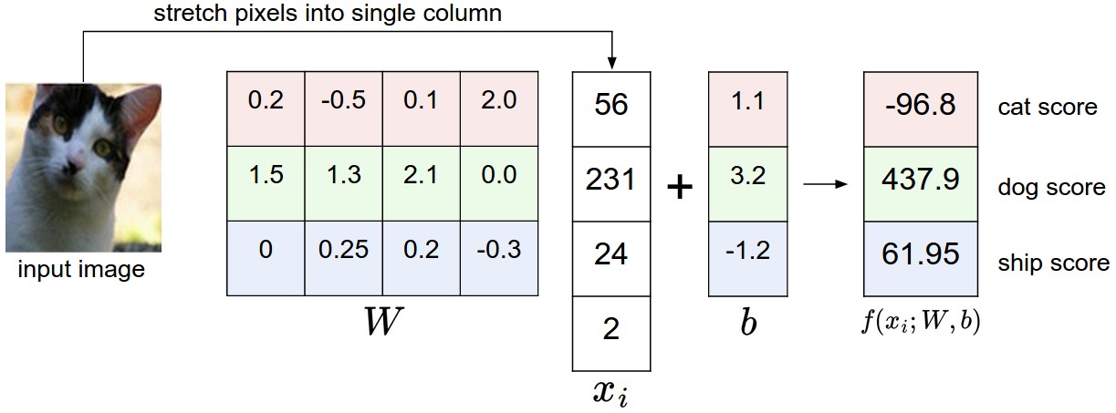An example of mapping an image to class scores. For the sake of visualization, we assume the image only has 4 pixels (4 monochrome pixels, we are not considering color channels in this example for brevity), and that we have 3 classes (red (cat), green (dog), blue (ship) class). (Clarification: in particular, the colors here simply indicate 3 classes and are not related to the RGB channels.) We stretch the image pixels into a column and perform matrix multiplication to get the scores for each class. Note that this particular set of weights W is not good at all: the weights assign our cat image a very low cat score. In particular, this set of weights seems convinced that it’s looking at a dog.

이미지를 클래스 점수로 보내는 예. 시각화를 위해 이미지에 픽셀이 4개뿐이라고 가정하고(간결함을 위해 색 채널은 고려하지 않은 흑백 픽셀 4개), 클래스는 3개(빨강은 cat, 초록은 dog, 파랑은 ship)라고 하자. (참고: 여기서 색은 단지 세 클래스를 구분하기 위한 것이고 RGB 채널과는 무관하다.) 이미지 픽셀을 하나의 열로 펼친 다음 행렬 곱을 해서 각 클래스의 점수를 얻는다. 이 가중치 W는 전혀 좋지 않다는 점에 주목하자. 고양이 이미지에 아주 낮은 고양이 점수를 매기고 있다. 특히 이 가중치는 지금 보고 있는 것이 개라고 확신하는 듯하다.

Analogy of images as high-dimensional points. Since the images are stretched into high-dimensional column vectors, we can interpret each image as a single point in this space (e.g. each image in CIFAR-10 is a point in 3072-dimensional space of 32x32x3 pixels). Analogously, the entire dataset is a (labeled) set of points.

이미지를 고차원 공간의 점으로 보는 비유. 이미지를 고차원 열벡터로 펼쳤으므로 각 이미지를 이 공간의 점 하나로 볼 수 있다(예컨대 CIFAR-10의 각 이미지는 32x32x3 픽셀이 이루는 3072차원 공간의 한 점이다). 같은 식으로 데이터셋 전체는 레이블이 달린 점들의 집합이 된다.

Since we defined the score of each class as a weighted sum of all image pixels, each class score is a linear function over this space. We cannot visualize 3072-dimensional spaces, but if we imagine squashing all those dimensions into only two dimensions, then we can try to visualize what the classifier might be doing:

각 클래스의 점수를 모든 이미지 픽셀의 가중합으로 정의했으므로 각 클래스 점수는 이 공간 위의 선형 함수다. 3072차원 공간을 눈으로 볼 수는 없지만, 그 모든 차원을 2차원으로 눌러 담았다고 상상하면 분류기가 무엇을 하고 있는지 그려볼 수 있다.

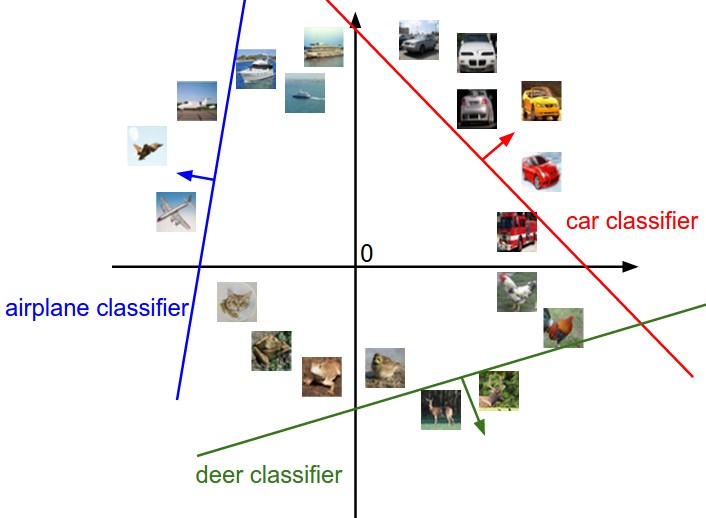Cartoon representation of the image space, where each image is a single point, and three classifiers are visualized. Using the example of the car classifier (in red), the red line shows all points in the space that get a score of zero for the car class. The red arrow shows the direction of increase, so all points to the right of the red line have positive (and linearly increasing) scores, and all points to the left have a negative (and linearly decreasing) scores.

이미지 공간을 만화처럼 나타낸 그림. 각 이미지는 점 하나이고 분류기 세 개가 그려져 있다. 빨간색 자동차 분류기를 예로 들면, 빨간 직선은 자동차 클래스 점수가 0이 되는 공간상의 모든 점이다. 빨간 화살표는 점수가 커지는 방향이므로 빨간 선 오른쪽의 모든 점은 양수 점수를 가지며 선형으로 커지고, 왼쪽의 모든 점은 음수 점수를 가지며 선형으로 작아진다.

As we saw above, every row of \(W\) is a classifier for one of the classes. The geometric interpretation of these numbers is that as we change one of the rows of \(W\), the corresponding line in the pixel space will rotate in different directions. The biases \(b\), on the other hand, allow our classifiers to translate the lines. In particular, note that without the bias terms, plugging in \(x_i = 0\) would always give score of zero regardless of the weights, so all lines would be forced to cross the origin.

앞에서 봤듯 \(W\)의 각 행은 클래스 하나에 대한 분류기다. 이 숫자들의 기하학적 의미는, \(W\)의 한 행을 바꾸면 픽셀 공간에서 그에 대응하는 직선이 이런저런 방향으로 회전한다는 것이다. 반면 편향 \(b\)는 그 직선을 평행이동시킨다. 특히 편향 항이 없다면 \(x_i = 0\)을 넣었을 때 가중치가 무엇이든 점수가 늘 0이 되므로, 모든 직선이 원점을 지나야만 한다는 점에 주목하자.

Interpretation of linear classifiers as template matching. Another interpretation for the weights \(W\) is that each row of \(W\) corresponds to a template (or sometimes also called a prototype) for one of the classes. The score of each class for an image is then obtained by comparing each template with the image using an inner product (or dot product) one by one to find the one that “fits” best. With this terminology, the linear classifier is doing template matching, where the templates are learned. Another way to think of it is that we are still effectively doing Nearest Neighbor, but instead of having thousands of training images we are only using a single image per class (although we will learn it, and it does not necessarily have to be one of the images in the training set), and we use the (negative) inner product as the distance instead of the L1 or L2 distance.

선형 분류기를 템플릿 매칭으로 보는 해석. 가중치 \(W\)를 보는 또 다른 방법은 \(W\)의 각 행을 클래스 하나에 대한 템플릿(프로토타입이라고도 한다)으로 보는 것이다. 그러면 어떤 이미지에 대한 각 클래스의 점수는 템플릿을 이미지와 하나씩 내적해서 어느 것이 가장 잘 “맞는지” 찾는 것으로 얻어진다. 이 용어를 쓰면 선형 분류기는 템플릿 매칭을 하고 있고, 그 템플릿은 학습으로 얻어진 것이다. 달리 보면 여전히 최근접 이웃을 하고 있는 셈인데, 다만 학습 이미지 수천 장 대신 클래스당 이미지 한 장만 쓰고(그마저도 학습으로 얻은 것이라 학습 집합 안의 이미지일 필요는 없다), 거리로는 L1이나 L2 거리 대신 내적에 음수를 붙인 값을 쓴다.

Skipping ahead a bit: Example learned weights at the end of learning for CIFAR-10. Note that, for example, the ship template contains a lot of blue pixels as expected. This template will therefore give a high score once it is matched against images of ships on the ocean with an inner product.

조금 앞서 가보면: CIFAR-10에서 학습이 끝났을 때 얻어진 가중치의 예. 예를 들어 배 템플릿에는 예상대로 파란 픽셀이 많다. 따라서 바다 위의 배 이미지와 내적하면 이 템플릿은 높은 점수를 낸다.

Additionally, note that the horse template seems to contain a two-headed horse, which is due to both left and right facing horses in the dataset. The linear classifier merges these two modes of horses in the data into a single template. Similarly, the car classifier seems to have merged several modes into a single template which has to identify cars from all sides, and of all colors. In particular, this template ended up being red, which hints that there are more red cars in the CIFAR-10 dataset than of any other color. The linear classifier is too weak to properly account for different-colored cars, but as we will see later neural networks will allow us to perform this task. Looking ahead a bit, a neural network will be able to develop intermediate neurons in its hidden layers that could detect specific car types (e.g. green car facing left, blue car facing front, etc.), and neurons on the next layer could combine these into a more accurate car score through a weighted sum of the individual car detectors.

또한 말 템플릿에는 머리가 둘 달린 말이 들어 있는 듯한데, 데이터셋에 왼쪽을 보는 말과 오른쪽을 보는 말이 둘 다 있기 때문이다. 선형 분류기는 데이터에 있는 이 두 가지 양상을 템플릿 하나로 합쳐버린다. 마찬가지로 자동차 분류기도 온갖 방향과 온갖 색의 자동차를 하나의 템플릿으로 알아보아야 하다 보니 여러 양상이 뭉뚱그려진 것으로 보인다. 특히 이 템플릿이 붉은색이 된 것은 CIFAR-10 데이터셋에 다른 어떤 색보다 빨간 자동차가 많다는 힌트다. 선형 분류기는 색이 다른 자동차들을 제대로 다루기에는 너무 약하지만, 뒤에서 보듯 신경망을 쓰면 이 일을 해낼 수 있다. 조금 앞서 가보면, 신경망은 은닉층에 특정 자동차 유형(예: 왼쪽을 보는 초록 자동차, 정면을 보는 파란 자동차 등)을 검출하는 중간 뉴런을 만들어낼 수 있고, 다음 층의 뉴런이 이런 개별 자동차 검출기들을 가중합해 더 정확한 자동차 점수로 합칠 수 있다.

Bias trick. Before moving on we want to mention a common simplifying trick to representing the two parameters \(W,b\) as one. Recall that we defined the score function as:

\[f(x_i, W, b) = W x_i + b\]

편향 트릭(bias trick). 넘어가기 전에 두 매개변수 \(W,b\)를 하나로 표현하는, 흔히 쓰는 단순화 트릭을 언급해둔다. 앞에서 점수 함수를 다음과 같이 정의했다.

As we proceed through the material it is a little cumbersome to keep track of two sets of parameters (the biases \(b\) and weights \(W\)) separately. A commonly used trick is to combine the two sets of parameters into a single matrix that holds both of them by extending the vector \(x_i\) with one additional dimension that always holds the constant \(1\) - a default bias dimension. With the extra dimension, the new score function will simplify to a single matrix multiply:

\[f(x_i, W) = W x_i\]

진도를 나가다 보면 편향 \(b\)와 가중치 \(W\)라는 두 벌의 매개변수를 따로 관리하는 것이 조금 성가시다. 흔히 쓰는 트릭은 벡터 \(x_i\)에 항상 상수 \(1\)을 담는 차원 하나를 덧붙여, 두 벌의 매개변수를 그 둘을 모두 담는 행렬 하나로 합치는 것이다. 이 여분의 차원이 기본 편향 차원(bias dimension)이다. 차원 하나가 늘어나면 새 점수 함수는 행렬 곱 하나로 단순해진다.

With our CIFAR-10 example, \(x_i\) is now [3073 x 1] instead of [3072 x 1] - (with the extra dimension holding the constant 1), and \(W\) is now [10 x 3073] instead of [10 x 3072]. The extra column that \(W\) now corresponds to the bias \(b\). An illustration might help clarify:

CIFAR-10 예에서 \(x_i\)는 이제 [3072 x 1]이 아니라 [3073 x 1]이 되고(늘어난 차원에 상수 1이 들어간다), \(W\)는 [10 x 3072]가 아니라 [10 x 3073]이 된다. \(W\)에 늘어난 열이 편향 \(b\)에 해당한다. 그림으로 보면 이해가 쉬울 것이다.

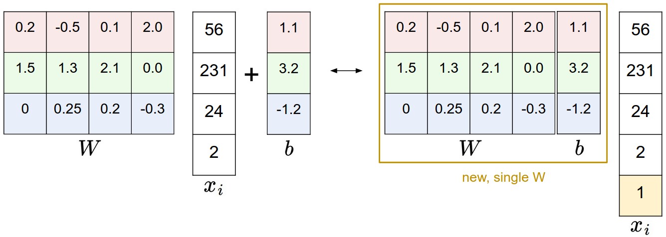Illustration of the bias trick. Doing a matrix multiplication and then adding a bias vector (left) is equivalent to adding a bias dimension with a constant of 1 to all input vectors and extending the weight matrix by 1 column - a bias column (right). Thus, if we preprocess our data by appending ones to all vectors we only have to learn a single matrix of weights instead of two matrices that hold the weights and the biases.

편향 트릭을 그림으로 나타낸 것. 행렬 곱을 한 다음 편향 벡터를 더하는 것(왼쪽)은, 모든 입력 벡터에 상수 1을 담은 편향 차원을 덧붙이고 가중치 행렬을 열 하나만큼, 즉 편향 열만큼 늘리는 것(오른쪽)과 같다. 따라서 데이터를 전처리해 모든 벡터에 1을 덧붙여두면, 가중치와 편향을 담은 두 개의 행렬 대신 가중치 행렬 하나만 학습하면 된다.

Image data preprocessing. As a quick note, in the examples above we used the raw pixel values (which range from [0…255]). In Machine Learning, it is a very common practice to always perform normalization of your input features (in the case of images, every pixel is thought of as a feature). In particular, it is important to center your data by subtracting the mean from every feature. In the case of images, this corresponds to computing a mean image across the training images and subtracting it from every image to get images where the pixels range from approximately [-127 … 127]. Further common preprocessing is to scale each input feature so that its values range from [-1, 1]. Of these, zero mean centering is arguably more important but we will have to wait for its justification until we understand the dynamics of gradient descent.

이미지 데이터 전처리. 짧게 짚어두면, 위 예에서는 원시 픽셀 값([0…255] 범위)을 그대로 썼다. 머신러닝에서는 입력 특징을 항상 정규화(normalization)하는 것이 아주 일반적인 관례다(이미지의 경우 픽셀 하나하나를 특징으로 본다). 특히 모든 특징에서 평균을 빼서 데이터를 중심에 맞추는 것이 중요하다. 이미지라면 학습 이미지들에 걸쳐 평균 이미지를 계산한 다음 모든 이미지에서 그것을 빼는 것에 해당하며, 그러면 픽셀 값이 대략 [-127 … 127] 범위가 된다. 여기서 더 나아가 각 입력 특징의 값이 [-1, 1] 범위에 들어오도록 크기를 조정하는 것도 흔한 전처리다. 이 가운데 평균을 0으로 맞추는 쪽이 더 중요하다고 할 만하지만, 그 근거는 경사 하강법의 동역학을 이해하고 나서야 설명할 수 있다.

역주. 이 문단의 ‘정규화’는 normalization, 즉 입력 특징의 값 범위를 고르게 맞추는 전처리를 가리킨다. 바로 다음 절에 나오는 정규화(regularization)는 가중치가 커지지 않도록 손실 함수에 벌점을 더하는 전혀 다른 기법이다. 두 원어가 한국어로는 모두 ‘정규화’로 굳어져 있어, 이 시리즈에서는 헷갈릴 만한 자리마다 원어를 함께 적는다.

Loss function

In the previous section we defined a function from the pixel values to class scores, which was parameterized by a set of weights \(W\). Moreover, we saw that we don’t have control over the data \((x_i,y_i)\) (it is fixed and given), but we do have control over these weights and we want to set them so that the predicted class scores are consistent with the ground truth labels in the training data.

앞 절에서 픽셀 값에서 클래스 점수로 가는 함수를 정의했고, 이 함수는 가중치 \(W\)로 매개변수화되어 있었다. 또한 데이터 \((x_i,y_i)\)는 우리가 어쩔 수 없는 것이지만(고정되어 주어진다) 가중치는 우리가 정할 수 있으며, 예측된 클래스 점수가 학습 데이터의 ground truth 레이블과 들어맞도록 가중치를 정하고 싶다는 것도 봤다.

For example, going back to the example image of a cat and its scores for the classes “cat”, “dog” and “ship”, we saw that the particular set of weights in that example was not very good at all: We fed in the pixels that depict a cat but the cat score came out very low (-96.8) compared to the other classes (dog score 437.9 and ship score 61.95). We are going to measure our unhappiness with outcomes such as this one with a loss function (or sometimes also referred to as the cost function or the objective). Intuitively, the loss will be high if we’re doing a poor job of classifying the training data, and it will be low if we’re doing well.

예를 들어 고양이 이미지와 “cat”, “dog”, “ship” 클래스에 대한 점수 예로 돌아가 보면, 그 예에 쓰인 가중치는 전혀 좋지 않았다. 고양이가 찍힌 픽셀을 넣었는데 고양이 점수가 다른 클래스들(dog 437.9, ship 61.95)에 비해 아주 낮게(-96.8) 나왔다. 이런 결과에 대한 불만은 손실 함수로 잰다(비용 함수(cost function)나 목적 함수(objective)라고도 부른다). 직관적으로 학습 데이터를 잘 분류하지 못하면 손실이 크고, 잘하면 손실이 작다.

Multiclass Support Vector Machine loss

There are several ways to define the details of the loss function. As a first example we will first develop a commonly used loss called the Multiclass Support Vector Machine (SVM) loss. The SVM loss is set up so that the SVM “wants” the correct class for each image to a have a score higher than the incorrect classes by some fixed margin \(\Delta\). Notice that it’s sometimes helpful to anthropomorphise the loss functions as we did above: The SVM “wants” a certain outcome in the sense that the outcome would yield a lower loss (which is good).

손실 함수를 구체적으로 정의하는 방법은 여러 가지다. 첫 예로 널리 쓰이는 Multiclass Support Vector Machine(SVM) 손실을 만들어본다. SVM 손실은 SVM이 각 이미지의 정답 클래스 점수가 오답 클래스 점수보다 정해진 마진 \(\Delta\)만큼 높기를 “원하도록” 짜여 있다. 위에서처럼 손실 함수를 의인화하면 이해에 도움이 될 때가 있다. SVM이 어떤 결과를 “원한다”는 말은 그 결과가 더 낮은 손실을 낸다는, 그러니까 좋은 일이라는 뜻이다.

Let’s now get more precise. Recall that for the i-th example we are given the pixels of image \(x_i\) and the label \(y_i\) that specifies the index of the correct class. The score function takes the pixels and computes the vector \(f(x_i, W)\) of class scores, which we will abbreviate to \(s\) (short for scores). For example, the score for the j-th class is the j-th element: \(s_j = f(x_i, W)_j\). The Multiclass SVM loss for the i-th example is then formalized as follows:

\[L_i = \sum_{j\neq y_i} \max(0, s_j - s_{y_i} + \Delta)\]

이제 좀 더 정확하게 써보자. i번째 예제에 대해 이미지 픽셀 \(x_i\)와 정답 클래스의 인덱스를 가리키는 레이블 \(y_i\)가 주어진다는 것을 떠올리자. 점수 함수는 이 픽셀을 받아 클래스 점수 벡터 \(f(x_i, W)\)를 계산하는데, 이를 줄여서 \(s\)(scores)라고 쓴다. 예를 들어 j번째 클래스의 점수는 j번째 원소, 즉 \(s_j = f(x_i, W)_j\)다. 그러면 i번째 예제에 대한 Multiclass SVM 손실은 다음과 같이 정식화된다.

Example. Lets unpack this with an example to see how it works. Suppose that we have three classes that receive the scores \(s = [13, -7, 11]\), and that the first class is the true class (i.e. \(y_i = 0\)). Also assume that \(\Delta\) (a hyperparameter we will go into more detail about soon) is 10. The expression above sums over all incorrect classes (\(j \neq y_i\)), so we get two terms:

\[L_i = \max(0, -7 - 13 + 10) + \max(0, 11 - 13 + 10)\]

예시. 어떻게 동작하는지 예를 들어 풀어보자. 클래스가 셋이고 점수가 \(s = [13, -7, 11]\)로 나왔으며 첫 번째 클래스가 정답(즉 \(y_i = 0\))이라고 하자. 그리고 \(\Delta\)(곧 자세히 다룰 하이퍼파라미터다)는 10이라고 하자. 위 식은 오답 클래스 전부(\(j \neq y_i\))에 대해 더하므로 항이 두 개 나온다.

You can see that the first term gives zero since [-7 - 13 + 10] gives a negative number, which is then thresholded to zero with the \(max(0,-)\) function. We get zero loss for this pair because the correct class score (13) was greater than the incorrect class score (-7) by at least the margin 10. In fact the difference was 20, which is much greater than 10 but the SVM only cares that the difference is at least 10; Any additional difference above the margin is clamped at zero with the max operation. The second term computes [11 - 13 + 10] which gives 8. That is, even though the correct class had a higher score than the incorrect class (13 > 11), it was not greater by the desired margin of 10. The difference was only 2, which is why the loss comes out to 8 (i.e. how much higher the difference would have to be to meet the margin). In summary, the SVM loss function wants the score of the correct class \(y_i\) to be larger than the incorrect class scores by at least by \(\Delta\) (delta). If this is not the case, we will accumulate loss.

첫 번째 항은 [-7 - 13 + 10]이 음수이고 \(max(0,-)\) 함수가 이를 0으로 잘라내므로 0이 된다. 이 쌍에서 손실이 0인 이유는 정답 클래스 점수(13)가 오답 클래스 점수(-7)보다 마진 10 이상 높았기 때문이다. 실제 차이는 20으로 10보다 훨씬 크지만 SVM은 차이가 10 이상이기만 하면 그 이상은 신경 쓰지 않는다. 마진을 넘는 초과분은 max 연산으로 0에 눌린다. 두 번째 항은 [11 - 13 + 10]을 계산해 8이 된다. 즉 정답 클래스 점수가 오답 클래스 점수보다 높긴 했지만(13 > 11) 원하는 마진 10만큼 높지는 않았다. 차이가 2뿐이었고, 그래서 손실이 8로 나온 것이다(마진을 채우려면 차이가 얼마나 더 커야 하는지를 나타낸다). 정리하면 SVM 손실 함수는 정답 클래스 \(y_i\)의 점수가 오답 클래스 점수들보다 적어도 \(\Delta\)(델타)만큼 크기를 원한다. 그렇지 않으면 손실이 쌓인다.

Note that in this particular module we are working with linear score functions ( \(f(x_i; W) = W x_i\) ), so we can also rewrite the loss function in this equivalent form:

\[L_i = \sum_{j\neq y_i} \max(0, w_j^T x_i - w_{y_i}^T x_i + \Delta)\]

이 단원에서는 선형 점수 함수(\(f(x_i; W) = W x_i\))를 다루고 있으므로 손실 함수를 다음과 같은 동치인 형태로 다시 쓸 수도 있다.

where \(w_j\) is the j-th row of \(W\) reshaped as a column. However, this will not necessarily be the case once we start to consider more complex forms of the score function \(f\).

여기서 \(w_j\)는 \(W\)의 j번째 행을 열벡터로 바꾼 것이다. 다만 점수 함수 \(f\)의 형태가 더 복잡해지면 반드시 이렇게 쓸 수 있는 것은 아니다.

A last piece of terminology we’ll mention before we finish with this section is that the threshold at zero \(max(0,-)\) function is often called the hinge loss. You’ll sometimes hear about people instead using the squared hinge loss SVM (or L2-SVM), which uses the form \(max(0,-)^2\) that penalizes violated margins more strongly (quadratically instead of linearly). The unsquared version is more standard, but in some datasets the squared hinge loss can work better. This can be determined during cross-validation.

이 절을 마치기 전에 용어를 하나 더 짚어두면, 0에서 잘라내는 \(max(0,-)\) 함수를 흔히 hinge loss라고 부른다. 대신 squared hinge loss SVM(또는 L2-SVM)을 쓴다는 이야기도 종종 듣게 될 텐데, 이는 \(max(0,-)^2\) 형태를 써서 마진 위반에 선형이 아니라 이차로, 즉 더 세게 벌점을 준다. 제곱하지 않은 쪽이 더 표준적이지만 데이터셋에 따라서는 squared hinge loss가 더 잘 동작하기도 한다. 이는 교차 검증으로 정할 수 있다.

The loss function quantifies our unhappiness with predictions on the training set

손실 함수는 학습 집합에 대한 예측이 얼마나 마음에 들지 않는지를 수치로 잰다.

The Multiclass Support Vector Machine “wants” the score of the correct class to be higher than all other scores by at least a margin of delta. If any class has a score inside the red region (or higher), then there will be accumulated loss. Otherwise the loss will be zero. Our objective will be to find the weights that will simultaneously satisfy this constraint for all examples in the training data and give a total loss that is as low as possible.

Multiclass Support Vector Machine은 정답 클래스의 점수가 다른 모든 점수보다 적어도 델타만큼 높기를 “원한다”. 어떤 클래스든 빨간 영역 안에(또는 그보다 높은 곳에) 점수가 있으면 손실이 쌓이고, 그렇지 않으면 손실은 0이다. 우리 목표는 학습 데이터의 모든 예제에 대해 이 조건을 동시에 만족시키면서 전체 손실이 가능한 한 낮아지는 가중치를 찾는 것이다.

Regularization. There is one bug with the loss function we presented above. Suppose that we have a dataset and a set of parameters W that correctly classify every example (i.e. all scores are so that all the margins are met, and \(L_i = 0\) for all i). The issue is that this set of W is not necessarily unique: there might be many similar W that correctly classify the examples. One easy way to see this is that if some parameters W correctly classify all examples (so loss is zero for each example), then any multiple of these parameters \(\lambda W\) where \(\lambda > 1\) will also give zero loss because this transformation uniformly stretches all score magnitudes and hence also their absolute differences. For example, if the difference in scores between a correct class and a nearest incorrect class was 15, then multiplying all elements of W by 2 would make the new difference 30.

정규화(regularization). 위에서 제시한 손실 함수에는 버그가 하나 있다. 어떤 데이터셋과, 모든 예제를 올바르게 분류하는 매개변수 W가 있다고 하자(즉 모든 마진이 충족되어 모든 i에 대해 \(L_i = 0\)이다). 문제는 이런 W가 유일하지 않을 수 있다는 것이다. 예제를 올바르게 분류하는 비슷한 W가 여럿 있을 수 있다. 이를 쉽게 확인하는 방법 하나는, 어떤 매개변수 W가 모든 예제를 올바르게 분류한다면(즉 예제마다 손실이 0이라면) \(\lambda > 1\)인 \(\lambda W\) 역시 손실이 0이 된다는 것이다. 이 변환은 모든 점수의 크기를 똑같이 늘리므로 그 절대적인 차이도 함께 늘어나기 때문이다. 예를 들어 정답 클래스와 가장 가까운 오답 클래스의 점수 차이가 15였다면, W의 모든 원소에 2를 곱하면 그 차이는 30이 된다.

In other words, we wish to encode some preference for a certain set of weights W over others to remove this ambiguity. We can do so by extending the loss function with a regularization penalty \(R(W)\). The most common regularization penalty is the squared L2 norm that discourages large weights through an elementwise quadratic penalty over all parameters:

\[R(W) = \sum_k\sum_l W_{k,l}^2\]

다시 말해 이 모호함을 없애려면 어떤 가중치 W를 다른 것보다 선호한다는 기준을 손실 함수에 담아야 한다. 손실 함수에 정규화 벌점(regularization penalty) \(R(W)\)를 덧붙이면 된다. 가장 흔한 정규화 벌점은 제곱 L2 노름으로, 모든 매개변수에 원소별로 이차 벌점을 매겨 큰 가중치를 억제한다.

In the expression above, we are summing up all the squared elements of \(W\). Notice that the regularization function is not a function of the data, it is only based on the weights. Including the regularization penalty completes the full Multiclass Support Vector Machine loss, which is made up of two components: the data loss (which is the average loss \(L_i\) over all examples) and the regularization loss. That is, the full Multiclass SVM loss becomes:

\[L = \underbrace{ \frac{1}{N} \sum_i L_i }_\text{data loss} + \underbrace{ \lambda R(W) }_\text{regularization loss} \\\\\]

위 식은 \(W\)의 모든 원소를 제곱해 더한 것이다. 정규화 함수가 데이터의 함수가 아니라 오직 가중치만으로 결정된다는 점에 주목하자. 정규화 벌점을 포함시키면 Multiclass Support Vector Machine 손실이 완성되는데, 이는 두 부분으로 이루어진다. 모든 예제에 대한 \(L_i\)의 평균인 데이터 손실(data loss)과 정규화 손실(regularization loss)이다. 즉 전체 Multiclass SVM 손실은 다음과 같다.

Or expanding this out in its full form:

\[L = \frac{1}{N} \sum_i \sum_{j\neq y_i} \left[ \max(0, f(x_i; W)_j - f(x_i; W)_{y_i} + \Delta) \right] + \lambda \sum_k\sum_l W_{k,l}^2\]

혹은 이를 완전히 펼쳐 쓰면 다음과 같다.

Where \(N\) is the number of training examples. As you can see, we append the regularization penalty to the loss objective, weighted by a hyperparameter \(\lambda\). There is no simple way of setting this hyperparameter and it is usually determined by cross-validation.

여기서 \(N\)은 학습 예제의 개수다. 보다시피 정규화 벌점을 하이퍼파라미터 \(\lambda\)로 가중해 손실 목적 함수에 덧붙였다. 이 하이퍼파라미터를 정하는 간단한 방법은 없고 보통 교차 검증으로 결정한다.

In addition to the motivation we provided above there are many desirable properties to include the regularization penalty, many of which we will come back to in later sections. For example, it turns out that including the L2 penalty leads to the appealing max margin property in SVMs (See CS229 lecture notes for full details if you are interested).

위에서 든 동기 말고도 정규화 벌점을 넣는 데는 바람직한 성질이 여럿 있으며, 상당수는 뒤에서 다시 다룬다. 예를 들어 L2 벌점을 넣으면 SVM에서 max margin이라는 매력적인 성질이 따라 나온다(관심이 있다면 CS229 강의 노트에서 자세한 내용을 볼 수 있다).

The most appealing property is that penalizing large weights tends to improve generalization, because it means that no input dimension can have a very large influence on the scores all by itself. For example, suppose that we have some input vector \(x = [1,1,1,1]\) and two weight vectors \(w_1 = [1,0,0,0]\), \(w_2 = [0.25,0.25,0.25,0.25]\). Then \(w_1^Tx = w_2^Tx = 1\) so both weight vectors lead to the same dot product, but the L2 penalty of \(w_1\) is 1.0 while the L2 penalty of \(w_2\) is only 0.25. Therefore, according to the L2 penalty the weight vector \(w_2\) would be preferred since it achieves a lower regularization loss. Intuitively, this is because the weights in \(w_2\) are smaller and more diffuse. Since the L2 penalty prefers smaller and more diffuse weight vectors, the final classifier is encouraged to take into account all input dimensions to small amounts rather than a few input dimensions and very strongly. As we will see later in the class, this effect can improve the generalization performance of the classifiers on test images and lead to less overfitting.

가장 매력적인 성질은 큰 가중치에 벌점을 주면 일반화가 좋아지는 경향이 있다는 점이다. 어떤 입력 차원 하나가 점수에 아주 큰 영향을 혼자서 끼칠 수 없게 되기 때문이다. 예를 들어 입력 벡터 \(x = [1,1,1,1]\)과 두 가중치 벡터 \(w_1 = [1,0,0,0]\), \(w_2 = [0.25,0.25,0.25,0.25]\)가 있다고 하자. \(w_1^Tx = w_2^Tx = 1\)이므로 두 가중치 벡터의 내적 값은 같지만, \(w_1\)의 L2 벌점은 1.0인 반면 \(w_2\)의 L2 벌점은 0.25뿐이다. 따라서 L2 벌점 기준으로는 정규화 손실이 더 낮은 \(w_2\)가 선호된다. 직관적으로는 \(w_2\)의 가중치가 더 작고 더 고르게 퍼져 있기 때문이다. L2 벌점이 작고 고르게 퍼진 가중치 벡터를 선호하므로, 최종 분류기는 몇 개 입력 차원에 아주 강하게 의존하기보다 모든 입력 차원을 조금씩 고려하도록 유도된다. 수업 뒤쪽에서 보겠지만 이 효과는 테스트 이미지에 대한 분류기의 일반화 성능을 높이고 과적합을 줄일 수 있다.

Note that biases do not have the same effect since, unlike the weights, they do not control the strength of influence of an input dimension. Therefore, it is common to only regularize the weights \(W\) but not the biases \(b\). However, in practice this often turns out to have a negligible effect. Lastly, note that due to the regularization penalty we can never achieve loss of exactly 0.0 on all examples, because this would only be possible in the pathological setting of \(W = 0\).

편향은 가중치와 달리 입력 차원의 영향력 크기를 좌우하지 않으므로 같은 효과가 없다는 점에 유의하자. 그래서 가중치 \(W\)만 정규화하고 편향 \(b\)는 정규화하지 않는 것이 일반적이다. 다만 실제로는 이 차이가 거의 영향을 주지 않는 경우가 많다. 마지막으로, 정규화 벌점 때문에 모든 예제에서 손실이 정확히 0.0이 되는 일은 결코 일어날 수 없다는 점도 알아두자. 그것은 \(W = 0\)이라는 병적인 경우에만 가능하기 때문이다.

Code. Here is the loss function (without regularization) implemented in Python, in both unvectorized and half-vectorized form:

코드. 아래는 정규화를 뺀 손실 함수를 파이썬으로 구현한 것이다. 벡터화하지 않은 형태와 절반만 벡터화한 형태 두 가지다.

역주. 코드의 D = W.shape[0]은 입력의 차원이 아니라 클래스 개수, 즉 앞에서 K라고 쓴 값이다. 앞 절에서 D를 입력 차원으로 썼기 때문에 이름이 겹치니 혼동하지 말자. np는 numpy이며 이 조각에는 import가 생략되어 있다. 코드는 원문과의 대조를 위해 손대지 않고 그대로 실었다.

def L_i(x, y, W):
  """
  unvectorized version. Compute the multiclass svm loss for a single example (x,y)
  - x is a column vector representing an image (e.g. 3073 x 1 in CIFAR-10)
    with an appended bias dimension in the 3073-rd position (i.e. bias trick)
  - y is an integer giving index of correct class (e.g. between 0 and 9 in CIFAR-10)
  - W is the weight matrix (e.g. 10 x 3073 in CIFAR-10)
  """
  delta = 1.0 # see notes about delta later in this section
  scores = W.dot(x) # scores becomes of size 10 x 1, the scores for each class
  correct_class_score = scores[y]
  D = W.shape[0] # number of classes, e.g. 10
  loss_i = 0.0
  for j in range(D): # iterate over all wrong classes
    if j == y:
      # skip for the true class to only loop over incorrect classes
      continue
    # accumulate loss for the i-th example
    loss_i += max(0, scores[j] - correct_class_score + delta)
  return loss_i

def L_i_vectorized(x, y, W):
  """
  A faster half-vectorized implementation. half-vectorized
  refers to the fact that for a single example the implementation contains
  no for loops, but there is still one loop over the examples (outside this function)
  """
  delta = 1.0
  scores = W.dot(x)
  # compute the margins for all classes in one vector operation
  margins = np.maximum(0, scores - scores[y] + delta)
  # on y-th position scores[y] - scores[y] canceled and gave delta. We want
  # to ignore the y-th position and only consider margin on max wrong class
  margins[y] = 0
  loss_i = np.sum(margins)
  return loss_i

def L(X, y, W):
  """
  fully-vectorized implementation :
  - X holds all the training examples as columns (e.g. 3073 x 50,000 in CIFAR-10)
  - y is array of integers specifying correct class (e.g. 50,000-D array)
  - W are weights (e.g. 10 x 3073)
  """
  # evaluate loss over all examples in X without using any for loops
  # left as exercise to reader in the assignment

The takeaway from this section is that the SVM loss takes one particular approach to measuring how consistent the predictions on training data are with the ground truth labels. Additionally, making good predictions on the training set is equivalent to minimizing the loss.

이 절의 요점은 SVM 손실이 학습 데이터에 대한 예측이 ground truth 레이블과 얼마나 들어맞는지를 재는 한 가지 구체적인 방식이라는 것이다. 그리고 학습 집합에서 좋은 예측을 하는 것은 곧 이 손실을 최소화하는 것과 같다.

All we have to do now is to come up with a way to find the weights that minimize the loss.

이제 남은 일은 이 손실을 최소로 만드는 가중치를 찾는 방법을 마련하는 것뿐이다.

Practical Considerations

Setting Delta. Note that we brushed over the hyperparameter \(\Delta\) and its setting. What value should it be set to, and do we have to cross-validate it? It turns out that this hyperparameter can safely be set to \(\Delta = 1.0\) in all cases. The hyperparameters \(\Delta\) and \(\lambda\) seem like two different hyperparameters, but in fact they both control the same tradeoff: The tradeoff between the data loss and the regularization loss in the objective. The key to understanding this is that the magnitude of the weights \(W\) has direct effect on the scores (and hence also their differences): As we shrink all values inside \(W\) the score differences will become lower, and as we scale up the weights the score differences will all become higher. Therefore, the exact value of the margin between the scores (e.g. \(\Delta = 1\), or \(\Delta = 100\)) is in some sense meaningless because the weights can shrink or stretch the differences arbitrarily. Hence, the only real tradeoff is how large we allow the weights to grow (through the regularization strength \(\lambda\)).

델타 정하기. 하이퍼파라미터 \(\Delta\)와 그 설정을 그냥 지나쳤다. 어떤 값으로 두어야 하고, 교차 검증으로 정해야 할까? 결론부터 말하면 이 하이퍼파라미터는 어떤 경우에도 \(\Delta = 1.0\)으로 두어도 안전하다. \(\Delta\)와 \(\lambda\)는 서로 다른 두 하이퍼파라미터처럼 보이지만 사실 둘 다 같은 트레이드오프를 조절한다. 목적 함수 안에서 데이터 손실과 정규화 손실 사이의 트레이드오프다. 이를 이해하는 열쇠는 가중치 \(W\)의 크기가 점수에, 따라서 점수 차이에도 직접 영향을 준다는 점이다. \(W\) 안의 값을 모두 줄이면 점수 차이가 작아지고, 가중치를 키우면 점수 차이가 모두 커진다. 그러므로 점수 사이 마진의 정확한 값(예: \(\Delta = 1\)인지 \(\Delta = 100\)인지)은 어떤 의미에서 무의미하다. 가중치가 그 차이를 얼마든지 줄이거나 늘릴 수 있기 때문이다. 결국 진짜 트레이드오프는 정규화 세기 \(\lambda\)를 통해 가중치가 얼마나 커지도록 허용하느냐, 이것 하나뿐이다.

Relation to Binary Support Vector Machine. You may be coming to this class with previous experience with Binary Support Vector Machines, where the loss for the i-th example can be written as:

\[L_i = C \max(0, 1 - y_i w^Tx_i) + R(W)\]

이진 서포트 벡터 머신과의 관계. 이 수업에 오기 전에 이진 서포트 벡터 머신을 접해봤을 수도 있다. 거기서 i번째 예제의 손실은 다음과 같이 쓸 수 있다.

where \(C\) is a hyperparameter, and \(y_i \in \{ -1,1 \}\). You can convince yourself that the formulation we presented in this section contains the binary SVM as a special case when there are only two classes. That is, if we only had two classes then the loss reduces to the binary SVM shown above. Also, \(C\) in this formulation and \(\lambda\) in our formulation control the same tradeoff and are related through reciprocal relation \(C \propto \frac{1}{\lambda}\).

여기서 \(C\)는 하이퍼파라미터이고 \(y_i \in \{ -1,1 \}\)이다. 이 절에서 제시한 정식화가 클래스가 둘뿐일 때 이진 SVM을 특수한 경우로 포함한다는 것은 직접 확인해볼 수 있다. 즉 클래스가 두 개라면 손실은 위의 이진 SVM으로 환원된다. 또한 이 정식화의 \(C\)와 우리 정식화의 \(\lambda\)는 같은 트레이드오프를 조절하며 \(C \propto \frac{1}{\lambda}\)라는 역수 관계로 이어져 있다.

역주. 환원은 직접 해보면 금방 보인다. 클래스가 0번과 1번 둘뿐일 때 \(L_i = \max(0, w_j^T x_i - w_{y_i}^T x_i + \Delta)\)에서 \(j\)는 정답이 아닌 나머지 한 클래스다. 두 행의 차이를 \(w = w_1 - w_0\)으로 두면, 정답이 1번일 때는 \(L_i = \max(0, \Delta - w^T x_i)\), 정답이 0번일 때는 \(L_i = \max(0, \Delta + w^T x_i)\)가 된다. 정답을 \(\tilde{y}_i \in \{-1, 1\}\)로 표기하면 두 경우를 \(\max(0, \Delta - \tilde{y}_i w^T x_i)\) 하나로 묶을 수 있고, \(\Delta = 1\)을 넣으면 위의 이진 SVM 손실과 정확히 같아진다.

Aside: Optimization in primal. If you’re coming to this class with previous knowledge of SVMs, you may have also heard of kernels, duals, the SMO algorithm, etc. In this class (as is the case with Neural Networks in general) we will always work with the optimization objectives in their unconstrained primal form. Many of these objectives are technically not differentiable (e.g. the max(x,y) function isn’t because it has a kink when x=y), but in practice this is not a problem and it is common to use a subgradient.

곁가지: 원 문제에서의 최적화. SVM을 이미 알고 이 수업에 왔다면 커널, 쌍대 문제, SMO 알고리즘 같은 것도 들어봤을 것이다. 이 수업에서는 (신경망 전반이 그렇듯) 목적 함수를 제약이 없는 원 문제(primal) 형태 그대로 최적화한다. 이런 목적 함수 상당수는 엄밀히 말해 미분 가능하지 않지만(예컨대 max(x,y) 함수는 x=y에서 꺾임이 있어 미분 가능하지 않다) 실제로는 문제가 되지 않으며 보통 부분기울기(subgradient)를 쓴다.

Aside: Other Multiclass SVM formulations. It is worth noting that the Multiclass SVM presented in this section is one of few ways of formulating the SVM over multiple classes. Another commonly used form is the One-Vs-All (OVA) SVM which trains an independent binary SVM for each class vs. all other classes. Related, but less common to see in practice is also the All-vs-All (AVA) strategy. Our formulation follows the Weston and Watkins 1999 (pdf) version, which is a more powerful version than OVA (in the sense that you can construct multiclass datasets where this version can achieve zero data loss, but OVA cannot. See details in the paper if interested). The last formulation you may see is a Structured SVM, which maximizes the margin between the score of the correct class and the score of the highest-scoring incorrect runner-up class. Understanding the differences between these formulations is outside of the scope of the class. The version presented in these notes is a safe bet to use in practice, but the arguably simplest OVA strategy is likely to work just as well (as also argued by Rikin et al. 2004 in In Defense of One-Vs-All Classification (pdf)).

곁가지: Multiclass SVM의 다른 정식화들. 이 절에서 제시한 Multiclass SVM은 SVM을 여러 클래스로 확장하는 몇 안 되는 방법 중 하나라는 점을 짚어둘 만하다. 또 흔히 쓰이는 형태로는 각 클래스 대 나머지 전부에 대해 독립적인 이진 SVM을 학습시키는 One-Vs-All(OVA) SVM이 있다. 이와 관련되지만 실제로는 덜 보이는 것으로 All-vs-All(AVA) 전략도 있다. 우리가 쓴 정식화는 Weston and Watkins 1999 (pdf) 버전을 따르며 OVA보다 강력하다(이 버전은 데이터 손실을 0으로 만들 수 있지만 OVA는 그러지 못하는 다중 클래스 데이터셋을 만들 수 있다는 의미에서 그렇다. 관심이 있다면 논문에서 자세한 내용을 보라). 마지막으로 볼 수 있는 정식화는 Structured SVM으로, 정답 클래스 점수와 점수가 가장 높은 오답 클래스 점수 사이의 마진을 최대화한다. 이들 정식화의 차이를 이해하는 것은 이 수업의 범위를 벗어난다. 이 노트에서 제시한 버전은 실전에서 무난한 선택이지만, 가장 단순하다고 할 만한 OVA 전략도 그에 못지않게 잘 동작할 가능성이 크다(Rikin et al. 2004의 In Defense of One-Vs-All Classification (pdf)도 그렇게 주장한다).

보충: 델타와 람다가 같은 트레이드오프를 조절한다는 말

가중치를 \(c\)배로 키우면 모든 점수가 \(c\)배가 되므로 점수 차이도 \(c\)배가 된다. 그러니 마진 \(\Delta\)도 함께 \(c\)배로 키우면 데이터 손실이 통째로 \(c\)배가 될 뿐, 어느 가중치가 더 좋은지에 대한 판단은 하나도 바뀌지 않는다. 무작위 가중치로 직접 확인해보자.

import numpy as np

rng = np.random.default_rng(0)
W = rng.normal(size=(3, 4))   # 클래스 3개, 입력 차원 4
x = rng.normal(size=4)
y = 1                          # 정답 클래스

def svm_loss(W, x, y, delta):
    s = W.dot(x)
    margins = np.maximum(0, s - s[y] + delta)
    margins[y] = 0
    return np.sum(margins)

for c in [1.0, 2.0, 10.0]:
    data = svm_loss(c * W, x, y, c * 1.0)   # 가중치도 c배, 마진도 c배
    print(f"c = {c:5.1f}   delta = {c:5.1f}   data loss = {data:8.4f}   data loss / c = {data / c:.4f}")

c =   1.0   delta =   1.0   data loss =   5.8249   data loss / c = 5.8249
c =   2.0   delta =   2.0   data loss =  11.6498   data loss / c = 5.8249
c =  10.0   delta =  10.0   data loss =  58.2491   data loss / c = 5.8249

데이터 손실을 \(c\)로 나누면 언제나 같은 값이다. 즉 \((\Delta = 1, W)\)에서의 데이터 손실과 \((\Delta = c, cW)\)에서의 데이터 손실은 상수배 관계이므로 최소점의 위치가 같다. 달라지는 것은 정규화 항뿐이다. \(\lambda R(cW) = c^2 \lambda R(W)\)이므로, \(\Delta\)를 \(c\)배로 바꾸는 것은 \(\lambda\)를 조절하는 것으로 그대로 흡수된다. \(\Delta = 1.0\)으로 고정하고 \(\lambda\)만 교차 검증으로 찾아도 되는 이유가 이것이다.

Softmax classifier

It turns out that the SVM is one of two commonly seen classifiers. The other popular choice is the Softmax classifier, which has a different loss function. If you’ve heard of the binary Logistic Regression classifier before, the Softmax classifier is its generalization to multiple classes. Unlike the SVM which treats the outputs \(f(x_i,W)\) as (uncalibrated and possibly difficult to interpret) scores for each class, the Softmax classifier gives a slightly more intuitive output (normalized class probabilities) and also has a probabilistic interpretation that we will describe shortly. In the Softmax classifier, the function mapping \(f(x_i; W) = W x_i\) stays unchanged, but we now interpret these scores as the unnormalized log probabilities for each class and replace the hinge loss with a cross-entropy loss that has the form:

\[L_i = -\log\left(\frac{e^{f_{y_i}}}{ \sum_j e^{f_j} }\right) \hspace{0.5in} \text{or equivalently} \hspace{0.5in} L_i = -f_{y_i} + \log\sum_j e^{f_j}\]

SVM은 흔히 보는 두 분류기 중 하나다. 다른 하나로 널리 쓰이는 것이 Softmax 분류기이고, 손실 함수가 다르다. 이진 로지스틱 회귀 분류기를 들어봤다면, Softmax 분류기는 그것을 여러 클래스로 일반화한 것이다. SVM이 출력 \(f(x_i,W)\)를 각 클래스에 대한 (보정되지 않아 해석하기 어려울 수 있는) 점수로 다루는 것과 달리, Softmax 분류기는 조금 더 직관적인 출력, 즉 정규화된 클래스 확률을 내놓고 곧 설명할 확률적 해석도 가능하다. Softmax 분류기에서 매핑 \(f(x_i; W) = W x_i\)는 그대로 두되, 이 점수를 각 클래스의 정규화되지 않은 로그 확률로 해석하고 hinge loss 자리에 다음 형태의 교차 엔트로피 손실(cross-entropy loss)을 넣는다.

where we are using the notation \(f_j\) to mean the j-th element of the vector of class scores \(f\). As before, the full loss for the dataset is the mean of \(L_i\) over all training examples together with a regularization term \(R(W)\). The function \(f_j(z) = \frac{e^{z_j}}{\sum_k e^{z_k}}\) is called the softmax function: It takes a vector of arbitrary real-valued scores (in \(z\)) and squashes it to a vector of values between zero and one that sum to one. The full cross-entropy loss that involves the softmax function might look scary if you’re seeing it for the first time but it is relatively easy to motivate.

여기서 \(f_j\)는 클래스 점수 벡터 \(f\)의 j번째 원소를 뜻한다. 앞에서와 마찬가지로 데이터셋 전체의 손실은 모든 학습 예제에 대한 \(L_i\)의 평균에 정규화 항 \(R(W)\)를 더한 것이다. 함수 \(f_j(z) = \frac{e^{z_j}}{\sum_k e^{z_k}}\)를 softmax 함수라고 부른다. 임의의 실숫값 점수 벡터(\(z\))를 받아 0과 1 사이이면서 합이 1이 되는 값들의 벡터로 눌러 담는 함수다. softmax 함수가 들어간 교차 엔트로피 손실 전체는 처음 보면 무섭게 느껴질 수 있지만 어디서 온 것인지 이해하기는 비교적 쉽다.

Information theory view. The cross-entropy between a “true” distribution \(p\) and an estimated distribution \(q\) is defined as:

\[H(p,q) = - \sum_x p(x) \log q(x)\]

정보 이론의 관점. “참” 분포 \(p\)와 추정된 분포 \(q\) 사이의 교차 엔트로피는 다음과 같이 정의된다.

The Softmax classifier is hence minimizing the cross-entropy between the estimated class probabilities ( \(q = e^{f_{y_i}} / \sum_j e^{f_j}\) as seen above) and the “true” distribution, which in this interpretation is the distribution where all probability mass is on the correct class (i.e. \(p = [0, \ldots 1, \ldots, 0]\) contains a single 1 at the \(y_i\) -th position.). Moreover, since the cross-entropy can be written in terms of entropy and the Kullback-Leibler divergence as \(H(p,q) = H(p) + D_{KL}(p\vert{}\vert{}q)\), and the entropy of the delta function \(p\) is zero, this is also equivalent to minimizing the KL divergence between the two distributions (a measure of distance). In other words, the cross-entropy objective wants the predicted distribution to have all of its mass on the correct answer.

따라서 Softmax 분류기는 추정된 클래스 확률(위에서 본 \(q = e^{f_{y_i}} / \sum_j e^{f_j}\))과 “참” 분포 사이의 교차 엔트로피를 최소화하고 있는 것이다. 이 해석에서 참 분포란 확률 질량이 전부 정답 클래스에 몰려 있는 분포다(즉 \(p = [0, \ldots 1, \ldots, 0]\)은 \(y_i\)번째 자리에만 1이 하나 있다). 게다가 교차 엔트로피는 엔트로피와 쿨백-라이블러 발산을 써서 \(H(p,q) = H(p) + D_{KL}(p\vert{}\vert{}q)\)처럼 쓸 수 있고 델타 함수 \(p\)의 엔트로피는 0이므로, 이는 두 분포 사이의 KL 발산(거리의 척도)을 최소화하는 것과도 같다. 다시 말해 교차 엔트로피 목적 함수는 예측된 분포의 질량이 전부 정답에 몰리기를 원한다.

역주. 여기서 \(p\)는 정답 자리에만 1이 있는 원-핫 분포이므로 엔트로피 \(H(p) = -\sum_x p(x)\log p(x)\)가 0이다. \(1 \cdot \log 1 = 0\)이고 나머지 항은 확률이 0이라 아무것도 보태지 않는다. 그래서 \(H(p,q) = H(p) + D_{KL}(p\|q)\)에서 앞의 항이 사라지고, 교차 엔트로피를 줄이는 것이 곧 KL 발산 \(D_{KL}(p\|q)\)를 줄이는 것, 즉 추정 분포 \(q\)를 정답 분포 \(p\)에 가깝게 끌어당기는 것이 된다. \(D_{KL}\)은 거리처럼 쓰이지만 \(p\)와 \(q\)를 바꾸면 값이 달라지므로 엄밀한 의미의 거리는 아니다.

Probabilistic interpretation. Looking at the expression, we see that

\[P(y_i \mid x_i; W) = \frac{e^{f_{y_i}}}{\sum_j e^{f_j} }\]

확률적 해석. 식을 들여다보면 다음과 같은 값이 눈에 들어온다.

can be interpreted as the (normalized) probability assigned to the correct label \(y_i\) given the image \(x_i\) and parameterized by \(W\). To see this, remember that the Softmax classifier interprets the scores inside the output vector \(f\) as the unnormalized log probabilities. Exponentiating these quantities therefore gives the (unnormalized) probabilities, and the division performs the normalization so that the probabilities sum to one. In the probabilistic interpretation, we are therefore minimizing the negative log likelihood of the correct class, which can be interpreted as performing Maximum Likelihood Estimation (MLE). A nice feature of this view is that we can now also interpret the regularization term \(R(W)\) in the full loss function as coming from a Gaussian prior over the weight matrix \(W\), where instead of MLE we are performing the Maximum a posteriori (MAP) estimation. We mention these interpretations to help your intuitions, but the full details of this derivation are beyond the scope of this class.

이 값은 이미지 \(x_i\)가 주어지고 \(W\)로 매개변수화된 상황에서 정답 레이블 \(y_i\)에 할당된 (정규화된) 확률로 해석할 수 있다. 왜 그런지 보려면 Softmax 분류기가 출력 벡터 \(f\) 안의 점수를 정규화되지 않은 로그 확률로 해석한다는 것을 떠올리면 된다. 이 값들에 지수를 취하면 (정규화되지 않은) 확률이 되고, 나눗셈이 정규화를 수행해 확률의 합이 1이 되게 한다. 따라서 확률적 해석에서 우리는 정답 클래스의 음의 로그 가능도를 최소화하고 있는 셈이며, 이는 최대 가능도 추정(Maximum Likelihood Estimation, MLE)을 하는 것으로 볼 수 있다. 이 관점의 좋은 점은 전체 손실 함수의 정규화 항 \(R(W)\)를 가중치 행렬 \(W\)에 대한 가우시안 사전 분포에서 온 것으로 해석할 수 있다는 점이다. 그러면 MLE가 아니라 최대 사후 확률(Maximum a posteriori, MAP) 추정을 하는 셈이 된다. 직관을 돕기 위해 이런 해석들을 언급했지만 유도의 자세한 내용은 이 수업의 범위를 벗어난다.

Practical issues: Numeric stability. When you’re writing code for computing the Softmax function in practice, the intermediate terms \(e^{f_{y_i}}\) and \(\sum_j e^{f_j}\) may be very large due to the exponentials. Dividing large numbers can be numerically unstable, so it is important to use a normalization trick. Notice that if we multiply the top and bottom of the fraction by a constant \(C\) and push it into the sum, we get the following (mathematically equivalent) expression:

\[\frac{e^{f_{y_i}}}{\sum_j e^{f_j}} = \frac{Ce^{f_{y_i}}}{C\sum_j e^{f_j}} = \frac{e^{f_{y_i} + \log C}}{\sum_j e^{f_j + \log C}}\]

실전 문제: 수치 안정성. 실제로 Softmax 함수를 계산하는 코드를 쓸 때, 지수 때문에 중간 항 \(e^{f_{y_i}}\)와 \(\sum_j e^{f_j}\)가 아주 커질 수 있다. 큰 수끼리 나누는 것은 수치적으로 불안정할 수 있으므로 정규화(normalization) 트릭을 쓰는 것이 중요하다. 분자와 분모에 상수 \(C\)를 곱하고 그것을 합 안으로 밀어 넣으면 수학적으로 동치인 다음 식을 얻는다.

We are free to choose the value of \(C\). This will not change any of the results, but we can use this value to improve the numerical stability of the computation. A common choice for \(C\) is to set \(\log C = -\max_j f_j\). This simply states that we should shift the values inside the vector \(f\) so that the highest value is zero. In code:

\(C\)의 값은 자유롭게 고를 수 있다. 결과는 전혀 바뀌지 않지만 이 값을 이용해 계산의 수치 안정성을 높일 수 있다. \(C\)로 흔히 고르는 값은 \(\log C = -\max_j f_j\)가 되게 하는 것이다. 벡터 \(f\) 안의 값들을 가장 큰 값이 0이 되도록 평행이동시키라는 뜻이다. 코드로 쓰면 다음과 같다.

f = np.array([123, 456, 789]) # example with 3 classes and each having large scores
p = np.exp(f) / np.sum(np.exp(f)) # Bad: Numeric problem, potential blowup

# instead: first shift the values of f so that the highest number is 0:
f -= np.max(f) # f becomes [-666, -333, 0]
p = np.exp(f) / np.sum(np.exp(f)) # safe to do, gives the correct answer

Possibly confusing naming conventions. To be precise, the SVM classifier uses the hinge loss, or also sometimes called the max-margin loss. The Softmax classifier uses the cross-entropy loss. The Softmax classifier gets its name from the softmax function, which is used to squash the raw class scores into normalized positive values that sum to one, so that the cross-entropy loss can be applied. In particular, note that technically it doesn’t make sense to talk about the “softmax loss”, since softmax is just the squashing function, but it is a relatively commonly used shorthand.

헷갈리기 쉬운 이름들. 정확히 말하면 SVM 분류기는 hinge loss, 다른 이름으로 max-margin loss를 쓴다. Softmax 분류기는 교차 엔트로피 손실을 쓴다. Softmax 분류기라는 이름은 softmax 함수에서 왔다. 이 함수는 원시 클래스 점수를 합이 1인 양수 값들로 눌러 담아 교차 엔트로피 손실을 적용할 수 있게 해준다. 특히 엄밀히 따지면 “softmax 손실”이라는 말은 성립하지 않는다는 점에 주목하자. softmax는 눌러 담는 함수일 뿐이기 때문이다. 다만 줄임말로는 비교적 흔히 쓰인다.

SVM vs. Softmax

A picture might help clarify the distinction between the Softmax and SVM classifiers:

그림으로 보면 Softmax 분류기와 SVM 분류기의 차이가 분명해진다.

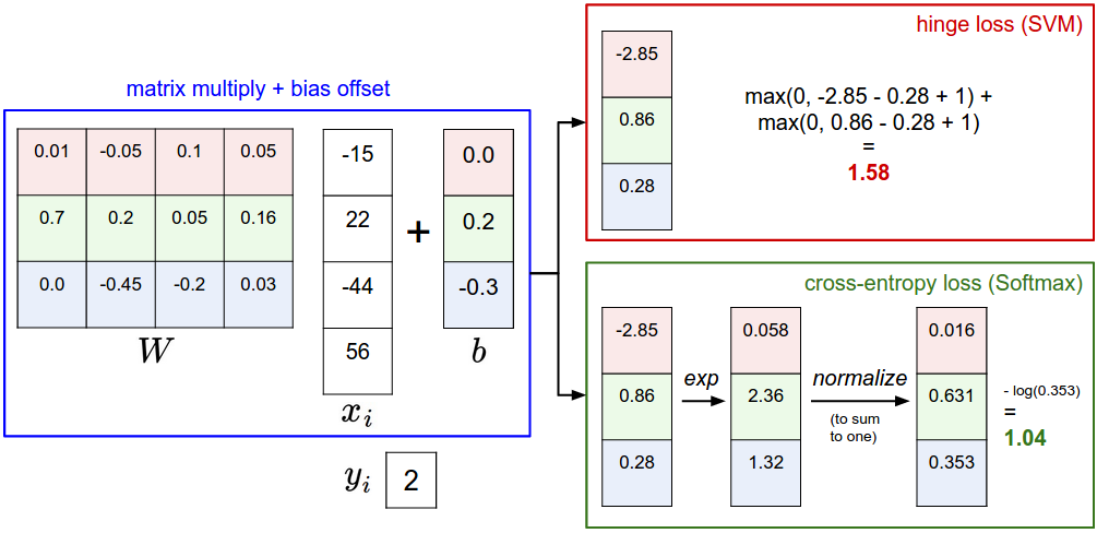Example of the difference between the SVM and Softmax classifiers for one datapoint. In both cases we compute the same score vector f (e.g. by matrix multiplication in this section). The difference is in the interpretation of the scores in f: The SVM interprets these as class scores and its loss function encourages the correct class (class 2, in blue) to have a score higher by a margin than the other class scores. The Softmax classifier instead interprets the scores as (unnormalized) log probabilities for each class and then encourages the (normalized) log probability of the correct class to be high (equivalently the negative of it to be low). The final loss for this example is 1.58 for the SVM and 1.04 (note this is 1.04 using the natural logarithm, not base 2 or base 10) for the Softmax classifier, but note that these numbers are not comparable; They are only meaningful in relation to loss computed within the same classifier and with the same data.

데이터 하나에 대해 SVM 분류기와 Softmax 분류기가 어떻게 다른지 보인 예. 두 경우 모두 같은 점수 벡터 f를 계산한다(이 절에서는 행렬 곱으로 얻는다). 차이는 f 안의 점수를 어떻게 해석하느냐에 있다. SVM은 이를 클래스 점수로 해석하고, 손실 함수는 정답 클래스(파란색 2번 클래스)의 점수가 다른 클래스 점수보다 마진만큼 높아지도록 유도한다. 반면 Softmax 분류기는 점수를 각 클래스의 (정규화되지 않은) 로그 확률로 해석하고, 정답 클래스의 (정규화된) 로그 확률이 높아지도록, 달리 말해 그 음수가 낮아지도록 유도한다. 이 예에서 최종 손실은 SVM이 1.58, Softmax가 1.04다(1.04는 밑이 2나 10이 아니라 자연로그로 계산한 값이다). 다만 이 두 숫자는 서로 비교할 수 있는 값이 아니다. 같은 분류기 안에서 같은 데이터로 계산한 손실끼리 비교할 때만 의미가 있다.

Softmax classifier provides “probabilities” for each class. Unlike the SVM which computes uncalibrated and not easy to interpret scores for all classes, the Softmax classifier allows us to compute “probabilities” for all labels. For example, given an image the SVM classifier might give you scores [12.5, 0.6, -23.0] for the classes “cat”, “dog” and “ship”. The softmax classifier can instead compute the probabilities of the three labels as [0.9, 0.09, 0.01], which allows you to interpret its confidence in each class. The reason we put the word “probabilities” in quotes, however, is that how peaky or diffuse these probabilities are depends directly on the regularization strength \(\lambda\) - which you are in charge of as input to the system. For example, suppose that the unnormalized log-probabilities for some three classes come out to be [1, -2, 0]. The softmax function would then compute:

\[[1, -2, 0] \rightarrow [e^1, e^{-2}, e^0] = [2.71, 0.14, 1] \rightarrow [0.7, 0.04, 0.26]\]

Softmax 분류기는 각 클래스에 대한 “확률”을 준다. SVM이 보정되지 않아 해석하기 어려운 점수를 모든 클래스에 대해 계산하는 것과 달리, Softmax 분류기는 모든 레이블에 대한 “확률”을 계산해준다. 예를 들어 어떤 이미지에 대해 SVM 분류기가 “cat”, “dog”, “ship” 클래스에 [12.5, 0.6, -23.0]이라는 점수를 줄 수 있다. Softmax 분류기라면 대신 세 레이블의 확률을 [0.9, 0.09, 0.01]로 계산할 수 있고, 그러면 각 클래스에 대한 확신도를 해석할 수 있다. 다만 “확률”에 따옴표를 친 이유는, 이 확률이 얼마나 뾰족하냐 퍼져 있느냐가 정규화 세기 \(\lambda\)에 직접 좌우되기 때문이다. 그리고 \(\lambda\)는 시스템에 입력으로 넣는 값이니 우리가 정하는 것이다. 예를 들어 어떤 세 클래스의 정규화되지 않은 로그 확률이 [1, -2, 0]으로 나왔다고 하자. 그러면 softmax 함수는 다음을 계산한다.

Where the steps taken are to exponentiate and normalize to sum to one. Now, if the regularization strength \(\lambda\) was higher, the weights \(W\) would be penalized more and this would lead to smaller weights. For example, suppose that the weights became one half smaller ([0.5, -1, 0]). The softmax would now compute:

\[[0.5, -1, 0] \rightarrow [e^{0.5}, e^{-1}, e^0] = [1.65, 0.37, 1] \rightarrow [0.55, 0.12, 0.33]\]

여기서 밟는 단계는 지수를 취한 다음 합이 1이 되도록 정규화하는 것이다. 이제 정규화 세기 \(\lambda\)가 더 컸다면 가중치 \(W\)에 벌점이 더 세게 매겨져 가중치가 더 작아졌을 것이다. 예를 들어 가중치가 절반으로 줄어 [0.5, -1, 0]이 되었다고 하자. 그러면 softmax는 다음을 계산한다.

where the probabilites are now more diffuse. Moreover, in the limit where the weights go towards tiny numbers due to very strong regularization strength \(\lambda\), the output probabilities would be near uniform. Hence, the probabilities computed by the Softmax classifier are better thought of as confidences where, similar to the SVM, the ordering of the scores is interpretable, but the absolute numbers (or their differences) technically are not.

이제 확률이 더 고르게 퍼졌다. 나아가 정규화 세기 \(\lambda\)가 아주 커서 가중치가 0에 가까워지는 극한에서는 출력 확률이 균등 분포에 가까워진다. 따라서 Softmax 분류기가 계산한 확률은 확신도로 이해하는 편이 낫다. SVM과 마찬가지로 점수의 순서는 해석할 수 있지만 절대적인 값이나 그 차이는 엄밀히 말해 해석할 수 없다.

In practice, SVM and Softmax are usually comparable. The performance difference between the SVM and Softmax are usually very small, and different people will have different opinions on which classifier works better. Compared to the Softmax classifier, the SVM is a more local objective, which could be thought of either as a bug or a feature. Consider an example that achieves the scores [10, -2, 3] and where the first class is correct. An SVM (e.g. with desired margin of \(\Delta = 1\)) will see that the correct class already has a score higher than the margin compared to the other classes and it will compute loss of zero. The SVM does not care about the details of the individual scores: if they were instead [10, -100, -100] or [10, 9, 9] the SVM would be indifferent since the margin of 1 is satisfied and hence the loss is zero. However, these scenarios are not equivalent to a Softmax classifier, which would accumulate a much higher loss for the scores [10, 9, 9] than for [10, -100, -100]. In other words, the Softmax classifier is never fully happy with the scores it produces: the correct class could always have a higher probability and the incorrect classes always a lower probability and the loss would always get better. However, the SVM is happy once the margins are satisfied and it does not micromanage the exact scores beyond this constraint. This can intuitively be thought of as a feature: For example, a car classifier which is likely spending most of its “effort” on the difficult problem of separating cars from trucks should not be influenced by the frog examples, which it already assigns very low scores to, and which likely cluster around a completely different side of the data cloud.

실제로 SVM과 Softmax는 대개 비슷하다. SVM과 Softmax의 성능 차이는 보통 아주 작고, 어느 분류기가 더 나은지는 사람마다 의견이 갈린다. Softmax 분류기와 비교하면 SVM은 더 국소적인 목적 함수인데, 이를 결함으로 볼 수도 있고 장점으로 볼 수도 있다. 점수가 [10, -2, 3]으로 나왔고 첫 번째 클래스가 정답인 예를 생각해보자. (예컨대 원하는 마진이 \(\Delta = 1\)인) SVM은 정답 클래스가 이미 다른 클래스들보다 마진 이상 높은 점수를 받았다고 보고 손실을 0으로 계산한다. SVM은 개별 점수의 세부에는 관심이 없다. 점수가 [10, -100, -100]이든 [10, 9, 9]든 마진 1이 충족되어 손실이 0이므로 SVM에게는 매한가지다. 그러나 Softmax 분류기에게는 두 상황이 같지 않다. Softmax는 [10, 9, 9]에 대해 [10, -100, -100]보다 훨씬 큰 손실을 쌓는다. 다시 말해 Softmax 분류기는 자기가 낸 점수에 결코 완전히 만족하지 않는다. 정답 클래스의 확률은 언제나 더 높아질 수 있고 오답 클래스의 확률은 언제나 더 낮아질 수 있으며, 그때마다 손실은 더 나아진다. 반면 SVM은 마진이 충족되는 순간 만족하고 그 제약을 넘어서까지 점수를 시시콜콜 따지지 않는다. 이는 직관적으로 장점으로 볼 수 있다. 예를 들어 자동차와 트럭을 구분하는 어려운 문제에 “노력”의 대부분을 쓰고 있을 자동차 분류기는, 이미 아주 낮은 점수를 주고 있고 데이터 구름의 전혀 다른 쪽에 몰려 있을 개구리 예제들에 휘둘리지 않아야 한다.

보충: 같은 점수에 SVM 손실과 Softmax 손실을 직접 매겨보기

바로 위 문단의 주장, 즉 SVM은 [10, -100, -100]과 [10, 9, 9]를 똑같이 보지만 Softmax는 그러지 않는다는 말을 숫자로 확인해보자.

import numpy as np

def svm_loss(s, y, delta=1.0):
    margins = np.maximum(0, s - s[y] + delta)
    margins[y] = 0
    return margins.sum()

def softmax_loss(s, y):
    z = s - s.max()                      # 수치 안정성을 위한 이동
    return -z[y] + np.log(np.exp(z).sum())

y = 0                                    # 첫 번째 클래스가 정답
for scores in ([10, -2, 3], [10, -100, -100], [10, 9, 9]):
    s = np.array(scores, dtype=float)
    print(f"{str(scores):<20} SVM = {svm_loss(s, y):.4f}   Softmax = {softmax_loss(s, y):.4f}")

[10, -2, 3]          SVM = 0.0000   Softmax = 0.0009
[10, -100, -100]     SVM = 0.0000   Softmax = 0.0000
[10, 9, 9]           SVM = 0.0000   Softmax = 0.5514

SVM 손실은 세 경우 모두 0이다. 마진 1이 이미 충족되었으니 그 뒤로는 관심을 끊는다. 반면 Softmax 손실은 [10, 9, 9]에서 0.5514까지 올라간다. 정답 확률이 아직 1에서 멀기 때문이다. 점수를 더 벌리면 손실이 계속 줄어들 여지가 남아 있다는 뜻이고, 이것이 “Softmax는 자기가 낸 점수에 결코 만족하지 않는다”는 말의 실제 모습이다.

Interactive web demo

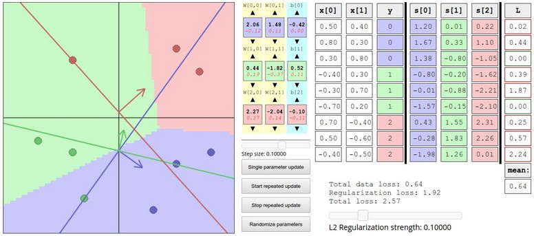We have written an interactive web demo to help your intuitions with linear classifiers. The demo visualizes the loss functions discussed in this section using a toy 3-way classification on 2D data. The demo also jumps ahead a bit and performs the optimization, which we will discuss in full detail in the next section.

선형 분류기에 대한 직관을 돕기 위해 대화형 웹 데모를 만들었다. 이 데모는 2차원 데이터에 대한 장난감 3-클래스 분류 문제로 이 절에서 다룬 손실 함수들을 시각화한다. 또한 조금 앞서 나가 최적화까지 수행하는데, 최적화는 다음 절에서 자세히 다룬다.

Summary

In summary,

정리하면 다음과 같다.

• We defined a score function from image pixels to class scores (in this section, a linear function that depends on weights W and biases b).
• Unlike kNN classifier, the advantage of this parametric approach is that once we learn the parameters we can discard the training data. Additionally, the prediction for a new test image is fast since it requires a single matrix multiplication with W, not an exhaustive comparison to every single training example.
• We introduced the bias trick, which allows us to fold the bias vector into the weight matrix for convenience of only having to keep track of one parameter matrix.
• We defined a loss function (we introduced two commonly used losses for linear classifiers: the SVM and the Softmax) that measures how compatible a given set of parameters is with respect to the ground truth labels in the training dataset. We also saw that the loss function was defined in such way that making good predictions on the training data is equivalent to having a small loss.

• 이미지 픽셀에서 클래스 점수로 가는 점수 함수를 정의했다(이 절에서는 가중치 W와 편향 b에 의존하는 선형 함수였다).
• kNN 분류기와 달리 이 매개변수적 접근법(parametric approach)의 장점은 매개변수를 배우고 나면 학습 데이터를 버릴 수 있다는 것이다. 게다가 새 테스트 이미지에 대한 예측이 빠르다. 모든 학습 예제와 하나하나 비교할 필요 없이 W와의 행렬 곱 한 번이면 되기 때문이다.
• 편향 벡터를 가중치 행렬에 접어 넣어 매개변수 행렬 하나만 관리하면 되게 해주는 편향 트릭을 소개했다.
• 주어진 매개변수가 학습 데이터셋의 ground truth 레이블과 얼마나 잘 맞는지를 재는 손실 함수를 정의했다(선형 분류기에 널리 쓰이는 두 손실, SVM과 Softmax를 소개했다). 또한 손실 함수가, 학습 데이터에서 좋은 예측을 하는 것이 곧 손실이 작은 것과 같아지도록 정의되었다는 점도 봤다.

We now saw one way to take a dataset of images and map each one to class scores based on a set of parameters, and we saw two examples of loss functions that we can use to measure the quality of the predictions. But how do we efficiently determine the parameters that give the best (lowest) loss? This process is optimization, and it is the topic of the next section.

이제 이미지 데이터셋을 받아 매개변수에 따라 각 이미지를 클래스 점수로 보내는 방법 하나를 봤고, 예측의 품질을 재는 데 쓸 수 있는 손실 함수의 예 두 가지도 봤다. 그렇다면 가장 좋은(가장 낮은) 손실을 내는 매개변수를 어떻게 효율적으로 찾을까? 이 과정이 최적화(optimization)이고, 다음 절의 주제다.

Further Reading

These readings are optional and contain pointers of interest.

아래 읽을거리는 선택 사항이며 관심이 갈 만한 것들을 가리킨다.

• Deep Learning using Linear Support Vector Machines from Charlie Tang 2013 presents some results claiming that the L2SVM outperforms Softmax.

• Charlie Tang의 2013년 논문 Deep Learning using Linear Support Vector Machines는 L2SVM이 Softmax를 능가한다고 주장하는 결과를 제시한다.