03. Optimization: Stochastic Gradient Descent
손실 함수 최적화, 수치적·해석적 기울기 계산, 경사 하강법과 mini-batch SGD.
원문: Optimization: Stochastic Gradient Descent — CS231n: Convolutional Neural Networks for Visual Recognition (Stanford University) · © 2015 Andrej Karpathy, MIT License
Introduction
In the previous section we introduced two key components in context of the image classification task:
지난 절에서 이미지 분류 작업의 맥락에서 핵심 요소 두 가지를 소개했다.
- A (parameterized) score function mapping the raw image pixels to class scores (e.g. a linear function)
- A loss function that measured the quality of a particular set of parameters based on how well the induced scores agreed with the ground truth labels in the training data. We saw that there are many ways and versions of this (e.g. Softmax/SVM).
- 원본 이미지 픽셀을 클래스 점수로 보내는 (매개변수화된) 점수 함수(예컨대 선형 함수)
- 어떤 매개변수 집합이 만들어낸 점수가 학습 데이터의 ground truth 레이블과 얼마나 잘 맞는지를 보고 그 매개변수 집합의 품질을 재는 손실 함수. 이 손실 함수에는 여러 방식과 변형이 있다는 것도 봤다(예컨대 Softmax/SVM).
Concretely, recall that the linear function had the form \(f(x_i, W) = W x_i\) and the SVM we developed was formulated as:
\[L = \frac{1}{N} \sum_i \sum_{j\neq y_i} \left[ \max(0, f(x_i; W)_j - f(x_i; W)_{y_i} + 1) \right] + \alpha R(W)\]
구체적으로, 선형 함수는 \(f(x_i, W) = W x_i\) 형태였고 우리가 만든 SVM은 다음과 같이 정식화되었다는 것을 떠올리자.
We saw that a setting of the parameters \(W\) that produced predictions for examples \(x_i\) consistent with their ground truth labels \(y_i\) would also have a very low loss \(L\). We are now going to introduce the third and last key component: optimization. Optimization is the process of finding the set of parameters \(W\) that minimize the loss function.
예제 \(x_i\)에 대해 그 ground truth 레이블 \(y_i\)와 들어맞는 예측을 내놓는 매개변수 \(W\)라면 손실 \(L\)도 아주 낮게 나온다는 것을 봤다. 이제 세 번째이자 마지막 핵심 요소인 최적화를 소개한다. 최적화는 손실 함수를 최소화하는 매개변수 집합 \(W\)를 찾아내는 과정이다.
Foreshadowing: Once we understand how these three core components interact, we will revisit the first component (the parameterized function mapping) and extend it to functions much more complicated than a linear mapping: First entire Neural Networks, and then Convolutional Neural Networks. The loss functions and the optimization process will remain relatively unchanged.
미리 말해두면: 이 세 핵심 요소가 어떻게 맞물리는지 이해하고 나면 첫 번째 요소인 매개변수화된 함수 매핑으로 돌아와, 그것을 선형 매핑보다 훨씬 복잡한 함수로 확장한다. 먼저 신경망 전체로, 그다음에는 합성곱 신경망으로 간다. 손실 함수와 최적화 과정은 거의 그대로 남는다.
Visualizing the loss function
The loss functions we’ll look at in this class are usually defined over very high-dimensional spaces (e.g. in CIFAR-10 a linear classifier weight matrix is of size [10 x 3073] for a total of 30,730 parameters), making them difficult to visualize. However, we can still gain some intuitions about one by slicing through the high-dimensional space along rays (1 dimension), or along planes (2 dimensions). For example, we can generate a random weight matrix \(W\) (which corresponds to a single point in the space), then march along a ray and record the loss function value along the way. That is, we can generate a random direction \(W_1\) and compute the loss along this direction by evaluating \(L(W + a W_1)\) for different values of \(a\). This process generates a simple plot with the value of \(a\) as the x-axis and the value of the loss function as the y-axis. We can also carry out the same procedure with two dimensions by evaluating the loss \(L(W + a W_1 + b W_2)\) as we vary \(a, b\). In a plot, \(a, b\) could then correspond to the x-axis and the y-axis, and the value of the loss function can be visualized with a color:
이 수업에서 다룰 손실 함수는 보통 아주 높은 차원의 공간 위에서 정의된다(예를 들어 CIFAR-10에서 선형 분류기의 가중치 행렬은 [10 x 3073] 크기이므로 매개변수가 모두 30,730개다). 그래서 눈으로 보기가 어렵다. 그래도 고차원 공간을 직선(1차원)이나 평면(2차원)을 따라 잘라보면 어느 정도 직관은 얻을 수 있다. 예를 들어 무작위 가중치 행렬 \(W\)(공간 속의 한 점에 해당한다)를 하나 만든 다음, 어떤 직선을 따라 걸어가며 손실 함수 값을 기록할 수 있다. 즉 무작위 방향 \(W_1\)을 하나 만들고 \(a\)를 여러 값으로 바꿔가며 \(L(W + a W_1)\)을 계산하면 그 방향을 따라간 손실을 알 수 있다. 이렇게 하면 \(a\) 값이 x축, 손실 함수 값이 y축인 간단한 그래프가 나온다. 같은 방법을 2차원으로도 할 수 있는데, \(a, b\)를 바꿔가며 손실 \(L(W + a W_1 + b W_2)\)를 계산하면 된다. 이때 \(a, b\)가 각각 x축과 y축이 되고 손실 함수 값은 색으로 나타낼 수 있다.
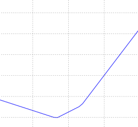
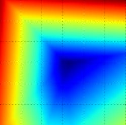
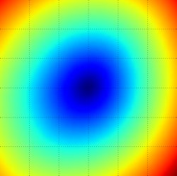 Loss function landscape for the Multiclass SVM (without regularization) for one single example (left,middle) and for a hundred examples (right) in CIFAR-10. Left: one-dimensional loss by only varying a. Middle, Right: two-dimensional loss slice, Blue = low loss, Red = high loss. Notice the piecewise-linear structure of the loss function. The losses for multiple examples are combined with average, so the bowl shape on the right is the average of many piece-wise linear bowls (such as the one in the middle).
정규화(regularization)를 뺀 Multiclass SVM의 손실 함수 지형. CIFAR-10에서 예제 한 개에 대한 것(왼쪽, 가운데)과 예제 백 개에 대한 것(오른쪽)이다. 왼쪽: a만 바꿔 얻은 1차원 손실. 가운데, 오른쪽: 2차원 손실 단면이며 파란색은 낮은 손실, 빨간색은 높은 손실이다. 손실 함수가 조각별 선형(piecewise-linear) 구조라는 점에 주목하자. 여러 예제의 손실은 평균으로 합쳐지므로 오른쪽의 그릇 모양은 (가운데 것과 같은) 조각별 선형 그릇을 여럿 평균 낸 결과다.
We can explain the piecewise-linear structure of the loss function by examining the math. For a single example we have:
\[L_i = \sum_{j\neq y_i} \left[ \max(0, w_j^Tx_i - w_{y_i}^Tx_i + 1) \right]\]
손실 함수가 왜 조각별 선형 구조인지는 식을 들여다보면 설명할 수 있다. 예제 하나에 대해서는 다음과 같다.
It is clear from the equation that the data loss for each example is a sum of (zero-thresholded due to the \(\max(0,-)\) function) linear functions of \(W\). Moreover, each row of \(W\) (i.e. \(w_j\)) sometimes has a positive sign in front of it (when it corresponds to a wrong class for an example), and sometimes a negative sign (when it corresponds to the correct class for that example). To make this more explicit, consider a simple dataset that contains three 1-dimensional points and three classes. The full SVM loss (without regularization) becomes:
\[\begin{align} L_0 = & \max(0, w_1^Tx_0 - w_0^Tx_0 + 1) + \max(0, w_2^Tx_0 - w_0^Tx_0 + 1) \\\\ L_1 = & \max(0, w_0^Tx_1 - w_1^Tx_1 + 1) + \max(0, w_2^Tx_1 - w_1^Tx_1 + 1) \\\\ L_2 = & \max(0, w_0^Tx_2 - w_2^Tx_2 + 1) + \max(0, w_1^Tx_2 - w_2^Tx_2 + 1) \\\\ L = & (L_0 + L_1 + L_2)/3 \end{align}\]
식을 보면 예제별 데이터 손실이 (\(\max(0,-)\) 함수 때문에 0에서 잘린) \(W\)의 선형 함수들을 더한 것임이 분명하다. 게다가 \(W\)의 각 행(즉 \(w_j\)) 앞에는 어떤 때는 양의 부호가 붙고(그 예제에서 오답 클래스에 해당할 때), 어떤 때는 음의 부호가 붙는다(그 예제에서 정답 클래스에 해당할 때). 이를 더 분명히 보기 위해 1차원 점 세 개와 클래스 세 개로 이루어진 간단한 데이터셋을 생각해보자. 정규화를 뺀 전체 SVM 손실은 다음과 같아진다.
Since these examples are 1-dimensional, the data \(x_i\) and weights \(w_j\) are numbers. Looking at, for instance, \(w_0\), some terms above are linear functions of \(w_0\) and each is clamped at zero. We can visualize this as follows:
이 예제들은 1차원이므로 데이터 \(x_i\)와 가중치 \(w_j\)는 그냥 숫자다. 예를 들어 \(w_0\)을 놓고 보면 위 식의 몇몇 항은 \(w_0\)의 선형 함수이고 각각은 0에서 잘려 있다. 이를 그림으로 나타내면 다음과 같다.
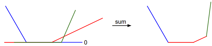 1-dimensional illustration of the data loss. The x-axis is a single weight and the y-axis is the loss. The data loss is a sum of multiple terms, each of which is either independent of a particular weight, or a linear function of it that is thresholded at zero. The full SVM data loss is a 30,730-dimensional version of this shape.
데이터 손실을 1차원으로 나타낸 그림. x축은 가중치 하나이고 y축은 손실이다. 데이터 손실은 여러 항을 더한 것이며, 각 항은 특정 가중치와 무관하거나 그 가중치의 선형 함수를 0에서 잘라낸 것이다. 전체 SVM 데이터 손실은 이 모양의 30,730차원 판이다.
As an aside, you may have guessed from its bowl-shaped appearance that the SVM cost function is an example of a convex function There is a large amount of literature devoted to efficiently minimizing these types of functions, and you can also take a Stanford class on the topic ( convex optimization ). Once we extend our score functions \(f\) to Neural Networks our objective functions will become non-convex, and the visualizations above will not feature bowls but complex, bumpy terrains.
곁가지로, 그릇 모양을 보고 짐작했을 수도 있지만 SVM 비용 함수는 볼록 함수의 한 예다. 이런 종류의 함수를 효율적으로 최소화하는 방법에 대해서는 방대한 문헌이 있고, 스탠퍼드에도 이를 다루는 수업(볼록 최적화)이 있다. 그러나 점수 함수 \(f\)를 신경망으로 확장하고 나면 목적 함수는 볼록하지 않게 되고, 위와 같은 시각화도 그릇이 아니라 울퉁불퉁하고 복잡한 지형으로 나타난다.
Non-differentiable loss functions. As a technical note, you can also see that the kinks in the loss function (due to the max operation) technically make the loss function non-differentiable because at these kinks the gradient is not defined. However, the subgradient still exists and is commonly used instead. In this class will use the terms subgradient and gradient interchangeably.
미분 가능하지 않은 손실 함수. 기술적인 이야기를 덧붙이면, max 연산 때문에 생기는 손실 함수의 꺾임은 엄밀히 말해 손실 함수를 미분 불가능하게 만든다. 그 꺾인 지점에서는 기울기가 정의되지 않기 때문이다. 하지만 부분기울기는 여전히 존재하고 보통 그것을 대신 쓴다. 이 수업에서는 부분기울기와 기울기를 구분 없이 섞어 쓴다.
Optimization
To reiterate, the loss function lets us quantify the quality of any particular set of weights W. The goal of optimization is to find W that minimizes the loss function. We will now motivate and slowly develop an approach to optimizing the loss function. For those of you coming to this class with previous experience, this section might seem odd since the working example we’ll use (the SVM loss) is a convex problem, but keep in mind that our goal is to eventually optimize Neural Networks where we can’t easily use any of the tools developed in the Convex Optimization literature.
다시 말하지만 손실 함수는 특정 가중치 집합 W의 품질을 수치로 재게 해준다. 최적화의 목표는 손실 함수를 최소화하는 W를 찾는 것이다. 이제 손실 함수를 최적화하는 방법을 동기부터 짚어가며 차근차근 만들어보겠다. 사전 지식을 갖고 이 수업에 온 사람에게는 이 절이 이상해 보일 수 있다. 예제로 쓸 SVM 손실이 볼록 문제이기 때문이다. 하지만 우리의 최종 목표는 신경망을 최적화하는 것이고, 거기서는 볼록 최적화 문헌의 도구를 그대로 가져다 쓸 수 없다는 점을 염두에 두자.
Strategy #1: A first very bad idea solution: Random search
Since it is so simple to check how good a given set of parameters W is, the first (very bad) idea that may come to mind is to simply try out many different random weights and keep track of what works best. This procedure might look as follows:
주어진 매개변수 집합 W가 얼마나 좋은지 확인하는 일은 아주 간단하므로, 가장 먼저 떠오르는 (아주 나쁜) 생각은 그저 서로 다른 무작위 가중치를 잔뜩 시도해보고 그중 가장 좋았던 것을 기록해두는 것이다. 절차는 다음과 같다.
역주. 이 절의 코드는 원문이 쓰인 시점의 Python 2 문법이라
print 'in attempt %d ...' % (...)처럼X_train과Xtr_cols,Y_test와Yte), 모두 같은 학습·테스트 데이터를 가리키는 것으로 읽으면 된다.np는numpy이고 import는 생략되어 있으며, 손실을 계산하는 함수L과 뒤에 나오는evaluate_gradient도 구현이 아니라 이름만 주어진 것이다. 코드는 원문과의 대조를 위해 손대지 않고 그대로 실었다.
1
2
3
4
5
6
7
8
9
10
11
12
13
14
15
16
17
18
19
20
21
22
# assume X_train is the data where each column is an example (e.g. 3073 x 50,000)
# assume Y_train are the labels (e.g. 1D array of 50,000)
# assume the function L evaluates the loss function

bestloss = float("inf") # Python assigns the highest possible float value
for num in range(1000):
  W = np.random.randn(10, 3073) * 0.0001 # generate random parameters
  loss = L(X_train, Y_train, W) # get the loss over the entire training set
  if loss < bestloss: # keep track of the best solution
    bestloss = loss
    bestW = W
  print 'in attempt %d the loss was %f, best %f' % (num, loss, bestloss)

# prints:
# in attempt 0 the loss was 9.401632, best 9.401632
# in attempt 1 the loss was 8.959668, best 8.959668
# in attempt 2 the loss was 9.044034, best 8.959668
# in attempt 3 the loss was 9.278948, best 8.959668
# in attempt 4 the loss was 8.857370, best 8.857370
# in attempt 5 the loss was 8.943151, best 8.857370
# in attempt 6 the loss was 8.605604, best 8.605604
# ... (trunctated: continues for 1000 lines)
In the code above, we see that we tried out several random weight vectors W, and some of them work better than others. We can take the best weights W found by this search and try it out on the test set:
위 코드에서는 무작위 가중치 벡터 W를 여럿 시도했고 그중 일부가 다른 것보다 낫다는 것을 볼 수 있다. 이 탐색으로 찾은 가장 좋은 가중치 W를 테스트 집합에 적용해볼 수 있다.
1
2
3
4
5
6
7
# Assume X_test is [3073 x 10000], Y_test [10000 x 1]
scores = Wbest.dot(Xte_cols) # 10 x 10000, the class scores for all test examples
# find the index with max score in each column (the predicted class)
Yte_predict = np.argmax(scores, axis = 0)
# and calculate accuracy (fraction of predictions that are correct)
np.mean(Yte_predict == Yte)
# returns 0.1555
With the best W this gives an accuracy of about 15.5%. Given that guessing classes completely at random achieves only 10%, that’s not a very bad outcome for a such a brain-dead random search solution!
가장 좋은 W로 얻은 정확도는 약 15.5%다. 클래스를 완전히 무작위로 찍으면 10%밖에 안 되니, 아무 생각 없는 무작위 탐색치고는 그리 나쁘지 않은 결과다.
Core idea: iterative refinement. Of course, it turns out that we can do much better. The core idea is that finding the best set of weights W is a very difficult or even impossible problem (especially once W contains weights for entire complex neural networks), but the problem of refining a specific set of weights W to be slightly better is significantly less difficult. In other words, our approach will be to start with a random W and then iteratively refine it, making it slightly better each time.
핵심 아이디어: 반복적 개선. 물론 훨씬 더 잘할 수 있다. 핵심 아이디어는 이렇다. 가장 좋은 가중치 집합 W를 찾는 것은 아주 어렵거나 심지어 불가능한 문제지만(특히 W가 복잡한 신경망 전체의 가중치를 담고 있다면 더욱 그렇다), 특정 가중치 집합 W를 조금 더 낫게 다듬는 문제는 그보다 훨씬 쉽다. 다시 말해 우리 접근법은 무작위 W에서 시작해 매번 조금씩 더 낫게 반복적으로 다듬어 가는 것이다.
Our strategy will be to start with random weights and iteratively refine them over time to get lower loss
우리 전략은 무작위 가중치에서 시작해 시간을 두고 반복적으로 다듬어 손실을 낮추는 것이다.
Blindfolded hiker analogy. One analogy that you may find helpful going forward is to think of yourself as hiking on a hilly terrain with a blindfold on, and trying to reach the bottom. In the example of CIFAR-10, the hills are 30,730-dimensional, since the dimensions of W are 10 x 3073. At every point on the hill we achieve a particular loss (the height of the terrain).
눈을 가린 등산객 비유. 앞으로 도움이 될 만한 비유가 하나 있다. 눈가리개를 하고 언덕진 지형을 걸으며 바닥에 닿으려 애쓰는 자신을 떠올려보자. CIFAR-10 예에서는 W의 크기가 10 x 3073이므로 이 언덕이 30,730차원이다. 언덕 위의 모든 지점에서 우리는 특정 손실 값(지형의 높이)을 얻는다.
Strategy #2: Random Local Search
The first strategy you may think of is to try to extend one foot in a random direction and then take a step only if it leads downhill. Concretely, we will start out with a random \(W\), generate random perturbations \(\delta W\) to it and if the loss at the perturbed \(W + \delta W\) is lower, we will perform an update. The code for this procedure is as follows:
가장 먼저 떠오르는 전략은 한쪽 발을 무작위 방향으로 뻗어보고 그쪽이 내리막일 때만 발을 딛는 것이다. 구체적으로는 무작위 \(W\)에서 시작해 무작위 교란 \(\delta W\)를 만들고, 교란된 \(W + \delta W\)에서의 손실이 더 낮으면 갱신을 수행한다. 이 절차의 코드는 다음과 같다.
1
2
3
4
5
6
7
8
9
10
W = np.random.randn(10, 3073) * 0.001 # generate random starting W
bestloss = float("inf")
for i in range(1000):
  step_size = 0.0001
  Wtry = W + np.random.randn(10, 3073) * step_size
  loss = L(Xtr_cols, Ytr, Wtry)
  if loss < bestloss:
    W = Wtry
    bestloss = loss
  print 'iter %d loss is %f' % (i, bestloss)
Using the same number of loss function evaluations as before (1000), this approach achieves test set classification accuracy of 21.4%. This is better, but still wasteful and computationally expensive.
앞과 같은 횟수(1000번)만큼 손실 함수를 계산했을 때 이 방법은 테스트 집합 분류 정확도 21.4%를 얻는다. 나아지긴 했지만 여전히 낭비가 심하고 계산 비용이 크다.
Strategy #3: Following the Gradient
In the previous section we tried to find a direction in the weight-space that would improve our weight vector (and give us a lower loss). It turns out that there is no need to randomly search for a good direction: we can compute the best direction along which we should change our weight vector that is mathematically guaranteed to be the direction of the steepest descent (at least in the limit as the step size goes towards zero). This direction will be related to the gradient of the loss function. In our hiking analogy, this approach roughly corresponds to feeling the slope of the hill below our feet and stepping down the direction that feels steepest.
앞 절에서는 가중치 벡터를 개선할(즉 손실을 낮출) 방향을 가중치 공간에서 찾으려 했다. 그런데 좋은 방향을 무작위로 찾아 헤맬 필요가 없다는 것이 밝혀진다. 가중치 벡터를 어느 쪽으로 바꿔야 하는지, 수학적으로 가장 가파른 내리막임이 보장된 최선의 방향을 계산할 수 있다(적어도 스텝 크기가 0으로 가는 극한에서는 그렇다). 이 방향은 손실 함수의 기울기(gradient)와 관련이 있다. 등산 비유로 보면 이 방법은 발밑 언덕의 경사를 더듬어 가장 가파르게 느껴지는 쪽으로 내려가는 것에 대략 해당한다.
In one-dimensional functions, the slope is the instantaneous rate of change of the function at any point you might be interested in. The gradient is a generalization of slope for functions that don’t take a single number but a vector of numbers. Additionally, the gradient is just a vector of slopes (more commonly referred to as derivatives) for each dimension in the input space. The mathematical expression for the derivative of a 1-D function with respect its input is:
\[\frac{df(x)}{dx} = \lim_{h\ \to 0} \frac{f(x + h) - f(x)}{h}\]
1차원 함수에서 기울기(slope)는 우리가 관심을 두는 어느 지점에서든 그 함수의 순간 변화율을 말한다. 기울기(gradient)는 숫자 하나가 아니라 숫자 벡터를 입력으로 받는 함수까지 이 개념을 일반화한 것이다. 또한 gradient는 입력 공간의 각 차원마다 구한 slope(더 흔히는 도함수라고 부른다)를 모아놓은 벡터일 뿐이다. 1차원 함수를 그 입력에 대해 미분한 것을 수학적으로 쓰면 다음과 같다.
역주. 이 문단에서 원문은 slope와 gradient를 구분해 쓰는데, 한국어로는 둘 다 ‘기울기’로 굳어져 있어 그대로 옮기면 구분이 사라진다. slope는 1차원 함수의 한 점에서의 기울기, 즉 숫자 하나다. gradient는 그 개념을 여러 변수로 확장한 것으로, 각 차원의 편미분을 모아놓은 벡터다. 이 포스트에서 아무 표시 없이 ‘기울기’라고 쓴 것은 모두 gradient를 가리키며, 원문이 둘을 나란히 대비하는 이 문단에서만 원어를 병기했다. 앞서 나온 정규화(regularization)와 정규화(normalization)의 겹침과 같은 종류다.
When the functions of interest take a vector of numbers instead of a single number, we call the derivatives partial derivatives, and the gradient is simply the vector of partial derivatives in each dimension.
관심 대상 함수가 숫자 하나가 아니라 숫자 벡터를 입력으로 받으면 그 도함수를 편미분이라고 부르며, gradient는 그저 각 차원에 대한 편미분을 모아놓은 벡터다.
Computing the gradient
There are two ways to compute the gradient: A slow, approximate but easy way (numerical gradient), and a fast, exact but more error-prone way that requires calculus (analytic gradient). We will now present both.
기울기를 계산하는 방법에는 두 가지가 있다. 느리고 근사적이지만 쉬운 방법(수치적 기울기)과, 빠르고 정확하지만 미적분이 필요해 실수하기 쉬운 방법(해석적 기울기)이다. 이제 둘 다 살펴본다.
Computing the gradient numerically with finite differences
The formula given above allows us to compute the gradient numerically. Here is a generic function that takes a function
f, a vectorxto evaluate the gradient on, and returns the gradient offatx:
위에서 준 공식으로 기울기를 수치적으로 계산할 수 있다. 아래는 함수 f와 기울기를 계산할 지점인 벡터 x를 받아 x에서의 f의 기울기를 돌려주는 범용 함수다.
1
2
3
4
5
6
7
8
9
10
11
12
13
14
15
16
17
18
19
20
21
22
23
24
25
26
27
def eval_numerical_gradient(f, x):
  """
  a naive implementation of numerical gradient of f at x
  - f should be a function that takes a single argument
  - x is the point (numpy array) to evaluate the gradient at
  """

  fx = f(x) # evaluate function value at original point
  grad = np.zeros(x.shape)
  h = 0.00001

  # iterate over all indexes in x
  it = np.nditer(x, flags=['multi_index'], op_flags=['readwrite'])
  while not it.finished:

    # evaluate function at x+h
    ix = it.multi_index
    old_value = x[ix]
    x[ix] = old_value + h # increment by h
    fxh = f(x) # evalute f(x + h)
    x[ix] = old_value # restore to previous value (very important!)

    # compute the partial derivative
    grad[ix] = (fxh - fx) / h # the slope
    it.iternext() # step to next dimension

  return grad
Following the gradient formula we gave above, the code above iterates over all dimensions one by one, makes a small change
halong that dimension and calculates the partial derivative of the loss function along that dimension by seeing how much the function changed. The variablegradholds the full gradient in the end.
위에서 제시한 기울기 공식을 따라, 이 코드는 모든 차원을 하나씩 훑으면서 그 차원 방향으로 작은 변화 h를 주고 함수 값이 얼마나 변했는지를 보아 그 차원에 대한 손실 함수의 편미분을 계산한다. 변수 grad가 마지막에 전체 기울기를 담는다.
Practical considerations. Note that in the mathematical formulation the gradient is defined in the limit as h goes towards zero, but in practice it is often sufficient to use a very small value (such as 1e-5 as seen in the example). Ideally, you want to use the smallest step size that does not lead to numerical issues. Additionally, in practice it often works better to compute the numeric gradient using the centered difference formula: \([f(x+h) - f(x-h)] / 2 h\) . See wiki for details.
실전에서 고려할 것. 수학적 정의에서 기울기는 h가 0으로 가는 극한으로 정의되지만, 실제로는 예제에서처럼 1e-5 같은 아주 작은 값을 쓰는 것으로 충분한 경우가 많다. 이상적으로는 수치적 문제를 일으키지 않는 한도에서 가장 작은 스텝 크기를 쓰는 것이 좋다. 또한 실전에서는 중심 차분 공식 \([f(x+h) - f(x-h)] / 2 h\)으로 수치적 기울기를 계산하는 편이 더 잘 동작하는 경우가 많다. 자세한 내용은 위키를 보라.
역주. 중심 차분이 더 정확한 이유는 테일러 전개로 보인다. \(f(x+h) = f(x) + f'(x)h + \frac{1}{2}f''(x)h^2 + O(h^3)\)이므로 앞의 단순한 차분 \([f(x+h)-f(x)]/h\)의 오차는 \(\frac{1}{2}f''(x)h\), 즉 \(O(h)\)다. 반면 \(f(x-h)\)까지 함께 쓰면 \(h^2\) 항이 서로 상쇄되어 \([f(x+h)-f(x-h)]/2h\)의 오차는 \(O(h^2)\)로 줄어든다. 같은 \(h\)로 훨씬 정확한 값을 얻는 대신 차원마다 함수를 두 번 계산해야 하므로 비용은 두 배가 된다.
We can use the function given above to compute the gradient at any point and for any function. Lets compute the gradient for the CIFAR-10 loss function at some random point in the weight space:
위에서 준 함수로 어떤 함수의 어떤 지점에서든 기울기를 계산할 수 있다. 가중치 공간의 무작위 지점에서 CIFAR-10 손실 함수의 기울기를 계산해보자.
1
2
3
4
5
6
7
8

# to use the generic code above we want a function that takes a single argument
# (the weights in our case) so we close over X_train and Y_train
def CIFAR10_loss_fun(W):
  return L(X_train, Y_train, W)

W = np.random.rand(10, 3073) * 0.001 # random weight vector
df = eval_numerical_gradient(CIFAR10_loss_fun, W) # get the gradient
The gradient tells us the slope of the loss function along every dimension, which we can use to make an update:
기울기는 모든 차원 방향으로 손실 함수가 얼마나 가파른지 알려주고, 우리는 이를 이용해 갱신을 수행할 수 있다.
1
2
3
4
5
6
7
8
9
10
11
12
13
14
15
16
17
18
19
20
21
22
loss_original = CIFAR10_loss_fun(W) # the original loss
print 'original loss: %f' % (loss_original, )

# lets see the effect of multiple step sizes
for step_size_log in [-10, -9, -8, -7, -6, -5,-4,-3,-2,-1]:
  step_size = 10 ** step_size_log
  W_new = W - step_size * df # new position in the weight space
  loss_new = CIFAR10_loss_fun(W_new)
  print 'for step size %f new loss: %f' % (step_size, loss_new)

# prints:
# original loss: 2.200718
# for step size 1.000000e-10 new loss: 2.200652
# for step size 1.000000e-09 new loss: 2.200057
# for step size 1.000000e-08 new loss: 2.194116
# for step size 1.000000e-07 new loss: 2.135493
# for step size 1.000000e-06 new loss: 1.647802
# for step size 1.000000e-05 new loss: 2.844355
# for step size 1.000000e-04 new loss: 25.558142
# for step size 1.000000e-03 new loss: 254.086573
# for step size 1.000000e-02 new loss: 2539.370888
# for step size 1.000000e-01 new loss: 25392.214036
Update in negative gradient direction. In the code above, notice that to compute
W_newwe are making an update in the negative direction of the gradientdfsince we wish our loss function to decrease, not increase.
기울기의 반대 방향으로 갱신하기. 위 코드에서 W_new를 계산할 때 기울기 df의 반대 방향으로 갱신한다는 점에 주목하자. 손실 함수가 커지는 것이 아니라 작아지길 원하기 때문이다.
Effect of step size. The gradient tells us the direction in which the function has the steepest rate of increase, but it does not tell us how far along this direction we should step. As we will see later in the course, choosing the step size (also called the learning rate) will become one of the most important (and most headache-inducing) hyperparameter settings in training a neural network. In our blindfolded hill-descent analogy, we feel the hill below our feet sloping in some direction, but the step length we should take is uncertain. If we shuffle our feet carefully we can expect to make consistent but very small progress (this corresponds to having a small step size). Conversely, we can choose to make a large, confident step in an attempt to descend faster, but this may not pay off. As you can see in the code example above, at some point taking a bigger step gives a higher loss as we “overstep”.
스텝 크기의 효과. 기울기는 함수가 가장 가파르게 증가하는 방향을 알려주지만, 그 방향으로 얼마나 멀리 가야 하는지는 알려주지 않는다. 수업 뒤쪽에서 보겠지만 스텝 크기(학습률이라고도 한다)를 고르는 일은 신경망을 학습시킬 때 가장 중요하면서도 가장 골치 아픈 하이퍼파라미터 설정 가운데 하나가 된다. 눈을 가린 채 언덕을 내려가는 비유로 보면, 발밑 언덕이 어느 쪽으로 기울어 있는지는 느껴지지만 보폭을 얼마로 잡아야 하는지는 알 수 없는 상황이다. 발을 조심조심 끌면 꾸준하지만 아주 조금씩만 나아갈 수 있다(스텝 크기가 작은 경우에 해당한다). 반대로 더 빨리 내려가려고 크고 자신 있게 한 걸음을 내디딜 수도 있지만, 그것이 늘 이득으로 돌아오지는 않는다. 위 코드 예제에서 보듯 어느 지점부터는 보폭을 키우면 “지나쳐버려” 손실이 오히려 높아진다.
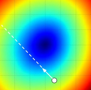 Visualizing the effect of step size. We start at some particular spot W and evaluate the gradient (or rather its negative - the white arrow) which tells us the direction of the steepest decrease in the loss function. Small steps are likely to lead to consistent but slow progress. Large steps can lead to better progress but are more risky. Note that eventually, for a large step size we will overshoot and make the loss worse. The step size (or as we will later call it - the learning rate) will become one of the most important hyperparameters that we will have to carefully tune.
스텝 크기의 효과를 시각화한 그림. 특정 지점 W에서 출발해 기울기를(정확히는 그 반대 방향, 즉 흰 화살표를) 계산하면 손실 함수가 가장 가파르게 감소하는 방향을 알 수 있다. 작은 보폭은 꾸준하지만 느린 진전으로 이어지기 쉽다. 큰 보폭은 더 빨리 나아갈 수 있지만 그만큼 위험하다. 스텝 크기가 크면 결국에는 지나쳐버려 손실이 더 나빠진다는 점에 유의하자. 스텝 크기(나중에는 학습률이라고 부를 것이다)는 우리가 신중히 조정해야 할 가장 중요한 하이퍼파라미터 가운데 하나가 된다.
A problem of efficiency. You may have noticed that evaluating the numerical gradient has complexity linear in the number of parameters. In our example we had 30730 parameters in total and therefore had to perform 30,731 evaluations of the loss function to evaluate the gradient and to perform only a single parameter update. This problem only gets worse, since modern Neural Networks can easily have tens of millions of parameters. Clearly, this strategy is not scalable and we need something better.
효율 문제. 수치적 기울기를 계산하는 비용이 매개변수 개수에 비례한다는 점을 눈치챘을 것이다. 우리 예에서는 매개변수가 모두 30,730개였으므로 기울기를 한 번 구해 매개변수를 단 한 번 갱신하기 위해 손실 함수를 30,731번 계산해야 했다. 현대의 신경망은 매개변수가 수천만 개에 이르기도 하므로 이 문제는 더 심각해지기만 한다. 이 전략은 분명 확장성이 없고, 더 나은 방법이 필요하다.
역주. 30,731번은 매개변수 30,730개마다 \(f(x+h)\)를 한 번씩 계산한 30,730번에, 기준값 \(f(x)\)를 구하는 한 번을 더한 수다. 위
eval_numerical_gradient코드에서fx = f(x)를 반복문 바깥에서 딱 한 번 계산하는 것이 그 한 번이다. 앞에서 권한 중심 차분을 쓰면 차원마다 두 번씩 계산해야 하므로 61,460번으로 늘어난다.
Computing the gradient analytically with Calculus
The numerical gradient is very simple to compute using the finite difference approximation, but the downside is that it is approximate (since we have to pick a small value of h, while the true gradient is defined as the limit as h goes to zero), and that it is very computationally expensive to compute. The second way to compute the gradient is analytically using Calculus, which allows us to derive a direct formula for the gradient (no approximations) that is also very fast to compute. However, unlike the numerical gradient it can be more error prone to implement, which is why in practice it is very common to compute the analytic gradient and compare it to the numerical gradient to check the correctness of your implementation. This is called a gradient check.
수치적 기울기는 유한 차분 근사로 계산하기가 아주 간단하지만, 근사값이라는 단점이 있고(작은 h 값을 골라야 하는데 참 기울기는 h가 0으로 가는 극한으로 정의된다) 계산 비용도 아주 크다. 기울기를 계산하는 두 번째 방법은 미적분을 이용해 해석적으로 구하는 것으로, 근사 없이 기울기의 직접적인 공식을 유도할 수 있고 계산도 아주 빠르다. 다만 수치적 기울기와 달리 구현에서 실수하기 쉬워서, 실전에서는 해석적 기울기를 계산한 뒤 수치적 기울기와 비교해 구현이 맞는지 확인하는 일이 아주 흔하다. 이를 gradient check라고 부른다.
Lets use the example of the SVM loss function for a single datapoint:
\[L_i = \sum_{j\neq y_i} \left[ \max(0, w_j^Tx_i - w_{y_i}^Tx_i + \Delta) \right]\]
데이터 포인트 하나에 대한 SVM 손실 함수를 예로 들어보자.
We can differentiate the function with respect to the weights. For example, taking the gradient with respect to \(w_{y_i}\) we obtain:
\[\nabla_{w_{y_i}} L_i = - \left( \sum_{j\neq y_i} \mathbb{1}(w_j^Tx_i - w_{y_i}^Tx_i + \Delta > 0) \right) x_i\]
이 함수를 가중치에 대해 미분할 수 있다. 예를 들어 \(w_{y_i}\)에 대한 기울기를 구하면 다음을 얻는다.
where \(\mathbb{1}\) is the indicator function that is one if the condition inside is true or zero otherwise. While the expression may look scary when it is written out, when you’re implementing this in code you’d simply count the number of classes that didn’t meet the desired margin (and hence contributed to the loss function) and then the data vector \(x_i\) scaled by this number is the gradient. Notice that this is the gradient only with respect to the row of \(W\) that corresponds to the correct class. For the other rows where \(j \neq y_i\) the gradient is:
\[\nabla_{w_j} L_i = \mathbb{1}(w_j^Tx_i - w_{y_i}^Tx_i + \Delta > 0) x_i\]
여기서 \(\mathbb{1}\)은 안의 조건이 참이면 1, 거짓이면 0인 지시 함수다. 펼쳐 쓴 식이 무섭게 보일 수 있지만, 코드로 구현할 때는 그저 원하는 마진을 채우지 못한(따라서 손실 함수에 기여한) 클래스의 개수를 세고, 데이터 벡터 \(x_i\)에 그 개수를 곱한 것이 곧 기울기다. 이것은 정답 클래스에 해당하는 \(W\)의 행에 대한 기울기일 뿐이라는 점에 주의하자. \(j \neq y_i\)인 나머지 행에 대한 기울기는 다음과 같다.
Once you derive the expression for the gradient it is straight-forward to implement the expressions and use them to perform the gradient update.
기울기의 식을 유도하고 나면 그 식을 구현해 기울기 갱신을 수행하는 것은 간단하다.
보충: 해석적 기울기가 맞는지 수치적 기울기로 확인하기
원문이 gradient check라고 부른 절차를 예제 하나짜리 SVM 손실에 직접 해보자. 바로 위에서 유도한 두 식, 즉 정답 클래스 행은 \(-\left( \sum_{j\neq y_i} \mathbb{1}(\cdot > 0) \right) x_i\)이고 나머지 행은 \(\mathbb{1}(\cdot > 0) x_i\)라는 것을 앞 절의 수치적 기울기와 맞춰보는 것이다.
1
2
3
4
5
6
7
8
9
10
11
12
13
14
15
16
17
18
19
20
21
22
23
24
25
26
27
28
29
30
31
32
33
34
35
36
37
38
39
40
41
42
43
44
45
46
47
48
49
import numpy as np

np.set_printoptions(precision=6, suppress=True)

rng = np.random.default_rng(1)
W = rng.normal(size=(3, 5)) * 0.1    # 클래스 3개, 입력 차원 5
x = rng.normal(size=5)
y = 2                                # 정답 클래스
delta = 1.0

def svm_loss_i(W):
    s = W.dot(x)
    margins = np.maximum(0, s - s[y] + delta)
    margins[y] = 0
    return margins.sum()

def analytic_grad(W):
    s = W.dot(x)
    margins = np.maximum(0, s - s[y] + delta)
    margins[y] = 0
    ind = (margins > 0).astype(float)   # 마진을 못 채운 오답 클래스에만 1
    dW = np.outer(ind, x)               # j != y_i 인 행: 1(...) * x_i
    dW[y] = -ind.sum() * x              # 정답 클래스 행: -(개수) * x_i
    return dW

def numeric_grad(f, W, h=1e-5):
    grad = np.zeros_like(W)
    it = np.nditer(W, flags=['multi_index'])
    while not it.finished:
        ix = it.multi_index
        old = W[ix]
        W[ix] = old + h; fph = f(W)
        W[ix] = old - h; fmh = f(W)
        W[ix] = old                        # 원래 값으로 반드시 되돌린다
        grad[ix] = (fph - fmh) / (2 * h)   # 중심 차분
        it.iternext()
    return grad

s = W.dot(x)
margins = np.maximum(0, s - s[y] + delta)
margins[y] = 0
ga, gn = analytic_grad(W), numeric_grad(svm_loss_i, W)

print("클래스 점수 s      =", s)
print("마진 위반량        =", margins, " -> 손실 L_i =", round(float(margins.sum()), 6))
print("마진을 못 채운 오답 클래스 수 =", int((margins > 0).sum()))
print("해석적 기울기:\n", ga)
print("수치적 기울기:\n", gn)
print("최대 절대 오차 =", float(np.max(np.abs(ga - gn))))
1
2
3
4
5
6
7
8
9
10
11
12
클래스 점수 s      = [ 0.092905 -0.028468  0.05055 ]
마진 위반량        = [1.042355 0.920982 0.      ]  -> 손실 L_i = 1.963337
마진을 못 채운 오답 클래스 수 = 2
해석적 기울기:
 [[ 0.598846  0.039722 -0.292457 -0.781908 -0.257192]
 [ 0.598846  0.039722 -0.292457 -0.781908 -0.257192]
 [-1.197692 -0.079444  0.584914  1.563817  0.514384]]
수치적 기울기:
 [[ 0.598846  0.039722 -0.292457 -0.781908 -0.257192]
 [ 0.598846  0.039722 -0.292457 -0.781908 -0.257192]
 [-1.197692 -0.079444  0.584914  1.563817  0.514384]]
최대 절대 오차 = 1.0487118118351901e-11
두 오답 클래스가 모두 마진을 못 채웠으므로 지시 함수는 둘 다 1이고, 그래서 0번 행과 1번 행이 똑같이 \(x_i\) 그 자체다. 정답 클래스인 2번 행은 그 개수 2를 곱하고 부호를 뒤집은 \(-2 x_i\)이며, 실제로 위의 두 행과 정확히 \(-2\)배 관계다. 세 행의 합이 0인 것도 여기서 나온다. 수치적 기울기와 비교했을 때 최대 오차는 1e-11 수준으로, 유한 차분 자체에서 나오는 오차 말고는 차이가 없다. 실전에서 해석적 기울기를 구현하고 나서 하는 일이 바로 이 대조다.
Gradient Descent
Now that we can compute the gradient of the loss function, the procedure of repeatedly evaluating the gradient and then performing a parameter update is called Gradient Descent. Its vanilla version looks as follows:
이제 손실 함수의 기울기를 계산할 수 있게 되었으니, 기울기를 되풀이해 계산하고 매개변수를 갱신하는 이 절차를 경사 하강법(Gradient Descent)이라고 부른다. 가장 기본이 되는 바닐라(vanilla) 버전은 다음과 같다.
1
2
3
4
5
# Vanilla Gradient Descent

while True:
  weights_grad = evaluate_gradient(loss_fun, data, weights)
  weights += - step_size * weights_grad # perform parameter update
This simple loop is at the core of all Neural Network libraries. There are other ways of performing the optimization (e.g. LBFGS), but Gradient Descent is currently by far the most common and established way of optimizing Neural Network loss functions. Throughout the class we will put some bells and whistles on the details of this loop (e.g. the exact details of the update equation), but the core idea of following the gradient until we’re happy with the results will remain the same.
이 단순한 반복문이 모든 신경망 라이브러리의 핵심이다. 최적화를 수행하는 다른 방법도 있지만(예컨대 LBFGS), 신경망 손실 함수를 최적화하는 방법으로는 경사 하강법이 현재까지 압도적으로 가장 흔하고 자리 잡은 방식이다. 수업 전반에 걸쳐 이 반복문의 세부에 이런저런 장식을 덧붙이겠지만(예컨대 갱신 식의 구체적인 형태), 결과가 만족스러워질 때까지 기울기를 따라간다는 핵심 생각은 그대로다.
Mini-batch gradient descent. In large-scale applications (such as the ILSVRC challenge), the training data can have on order of millions of examples. Hence, it seems wasteful to compute the full loss function over the entire training set in order to perform only a single parameter update. A very common approach to addressing this challenge is to compute the gradient over batches of the training data. For example, in current state of the art ConvNets, a typical batch contains 256 examples from the entire training set of 1.2 million. This batch is then used to perform a parameter update:
mini-batch 경사 하강법. (ILSVRC 챌린지 같은) 대규모 응용에서는 학습 데이터가 수백만 개에 이를 수 있다. 그러니 매개변수를 단 한 번 갱신하려고 학습 집합 전체에 대해 손실 함수를 계산하는 것은 낭비로 보인다. 이 문제를 해결하는 아주 흔한 접근법은 학습 데이터의 배치(batch) 단위로 기울기를 계산하는 것이다. 예를 들어 현재 최고 수준의 ConvNet에서는 120만 개의 전체 학습 집합에서 뽑은 예제 256개를 한 배치에 담는 것이 보통이다. 그리고 이 배치로 매개변수를 갱신한다.
1
2
3
4
5
6
# Vanilla Minibatch Gradient Descent

while True:
  data_batch = sample_training_data(data, 256) # sample 256 examples
  weights_grad = evaluate_gradient(loss_fun, data_batch, weights)
  weights += - step_size * weights_grad # perform parameter update
The reason this works well is that the examples in the training data are correlated. To see this, consider the extreme case where all 1.2 million images in ILSVRC are in fact made up of exact duplicates of only 1000 unique images (one for each class, or in other words 1200 identical copies of each image). Then it is clear that the gradients we would compute for all 1200 identical copies would all be the same, and when we average the data loss over all 1.2 million images we would get the exact same loss as if we only evaluated on a small subset of 1000. In practice of course, the dataset would not contain duplicate images, the gradient from a mini-batch is a good approximation of the gradient of the full objective. Therefore, much faster convergence can be achieved in practice by evaluating the mini-batch gradients to perform more frequent parameter updates.
이 방법이 잘 통하는 이유는 학습 데이터의 예제들이 서로 상관되어 있기 때문이다. 이를 확인하려면 극단적인 경우를 생각해보자. ILSVRC의 이미지 120만 장이 사실은 서로 다른 1000장(클래스마다 한 장씩, 다시 말해 각 이미지의 똑같은 사본 1200장)의 완전한 중복으로만 이루어져 있다고 하자. 그렇다면 똑같은 사본 1200장에 대해 계산한 기울기가 모두 같을 것이고, 120만 장 전체에 대해 데이터 손실을 평균 내면 1000장짜리 작은 부분집합만 계산했을 때와 정확히 같은 손실이 나온다는 것이 분명하다. 물론 실제 데이터셋에 중복 이미지가 들어 있지는 않겠지만, mini-batch에서 구한 기울기는 전체 목적 함수의 기울기를 잘 근사한다. 따라서 mini-batch 기울기를 계산해 매개변수를 더 자주 갱신하면 실전에서 훨씬 빠르게 수렴할 수 있다.
The extreme case of this is a setting where the mini-batch contains only a single example. This process is called Stochastic Gradient Descent (SGD) (or also sometimes on-line gradient descent). This is relatively less common to see because in practice due to vectorized code optimizations it can be computationally much more efficient to evaluate the gradient for 100 examples, than the gradient for one example 100 times. Even though SGD technically refers to using a single example at a time to evaluate the gradient, you will hear people use the term SGD even when referring to mini-batch gradient descent (i.e. mentions of MGD for “Minibatch Gradient Descent”, or BGD for “Batch gradient descent” are rare to see), where it is usually assumed that mini-batches are used. The size of the mini-batch is a hyperparameter but it is not very common to cross-validate it. It is usually based on memory constraints (if any), or set to some value, e.g. 32, 64 or 128. We use powers of 2 in practice because many vectorized operation implementations work faster when their inputs are sized in powers of 2.
이것의 극단적인 경우는 mini-batch에 예제가 단 하나만 들어 있는 설정이다. 이 과정을 Stochastic Gradient Descent (SGD)(또는 때때로 온라인(on-line) 경사 하강법)라고 부른다. 이것은 상대적으로 보기 드문데, 실제로는 벡터화된 코드 최적화 덕분에 예제 100개에 대한 기울기를 한 번에 계산하는 편이 예제 하나에 대한 기울기를 100번 계산하는 것보다 계산상 훨씬 효율적일 수 있기 때문이다. SGD는 엄밀히는 한 번에 예제 하나로 기울기를 계산하는 것을 가리키지만, 사람들이 mini-batch 경사 하강법을 가리킬 때도 SGD라는 말을 쓰는 것을 듣게 될 것이다(“Minibatch Gradient Descent”의 MGD나 “Batch gradient descent”의 BGD라는 표현은 좀처럼 보이지 않는다). 보통은 mini-batch를 쓴다고 전제하는 것이다. mini-batch의 크기는 하이퍼파라미터지만 이를 교차 검증으로 정하는 일은 그리 흔하지 않다. 보통은 (있다면) 메모리 제약을 기준으로 정하거나 32, 64, 128 같은 값으로 둔다. 실전에서 2의 거듭제곱을 쓰는 이유는 벡터화된 연산 구현 상당수가 입력 크기가 2의 거듭제곱일 때 더 빠르게 동작하기 때문이다.
Summary
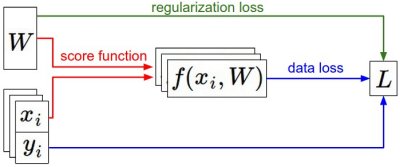 Summary of the information flow. The dataset of pairs of (x,y) is given and fixed. The weights start out as random numbers and can change. During the forward pass the score function computes class scores, stored in vector f. The loss function contains two components: The data loss computes the compatibility between the scores f and the labels y. The regularization loss is only a function of the weights. During Gradient Descent, we compute the gradient on the weights (and optionally on data if we wish) and use them to perform a parameter update during Gradient Descent.
정보 흐름을 정리한 그림. (x,y) 쌍으로 이루어진 데이터셋은 주어져 있고 고정되어 있다. 가중치는 무작위 값에서 시작하며 바뀔 수 있다. 순전파(forward pass) 동안 점수 함수가 클래스 점수를 계산해 벡터 f에 담는다. 손실 함수는 두 부분으로 이루어진다. 데이터 손실은 점수 f와 레이블 y가 얼마나 잘 맞는지를 계산한다. 정규화 손실은 오직 가중치만의 함수다. 경사 하강법을 수행하는 동안 우리는 가중치에 대한 기울기를(원한다면 데이터에 대한 기울기도) 계산하고 그것으로 매개변수를 갱신한다.
In this section,
이 절에서 다룬 내용은 다음과 같다.
- We developed the intuition of the loss function as a high-dimensional optimization landscape in which we are trying to reach the bottom. The working analogy we developed was that of a blindfolded hiker who wishes to reach the bottom. In particular, we saw that the SVM cost function is piece-wise linear and bowl-shaped.
- We motivated the idea of optimizing the loss function with iterative refinement, where we start with a random set of weights and refine them step by step until the loss is minimized.
- We saw that the gradient of a function gives the steepest ascent direction and we discussed a simple but inefficient way of computing it numerically using the finite difference approximation (the finite difference being the value of h used in computing the numerical gradient).
- We saw that the parameter update requires a tricky setting of the step size (or the learning rate) that must be set just right: if it is too low the progress is steady but slow. If it is too high the progress can be faster, but more risky. We will explore this tradeoff in much more detail in future sections.
- We discussed the tradeoffs between computing the numerical and analytic gradient. The numerical gradient is simple but it is approximate and expensive to compute. The analytic gradient is exact, fast to compute but more error-prone since it requires the derivation of the gradient with math. Hence, in practice we always use the analytic gradient and then perform a gradient check, in which its implementation is compared to the numerical gradient.
- We introduced the Gradient Descent algorithm which iteratively computes the gradient and performs a parameter update in loop.
- 손실 함수를, 우리가 바닥에 닿으려 애쓰는 고차원 최적화 지형으로 보는 직관을 세웠다. 이를 위해 쓴 비유는 바닥에 닿고자 하는, 눈을 가린 등산객이었다. 특히 SVM 비용 함수가 조각별 선형이고 그릇 모양이라는 것을 봤다.
- 무작위 가중치 집합에서 시작해 손실이 최소가 될 때까지 한 걸음씩 다듬어가는 반복적 개선으로 손실 함수를 최적화한다는 생각의 동기를 짚었다.
- 함수의 기울기가 가장 가파르게 상승하는 방향을 알려준다는 것을 봤고, 유한 차분 근사(유한 차분이란 수치적 기울기를 계산할 때 쓰는 h 값을 말한다)로 이를 수치적으로 계산하는, 간단하지만 비효율적인 방법을 이야기했다.
- 매개변수 갱신에는 스텝 크기(또는 학습률)를 까다롭게 맞춰야 한다는 것을 봤다. 너무 작으면 진전이 꾸준하지만 느리고, 너무 크면 더 빠를 수 있지만 그만큼 위험하다. 이 트레이드오프는 뒤에서 훨씬 자세히 다룬다.
- 수치적 기울기와 해석적 기울기를 계산하는 것 사이의 트레이드오프를 논의했다. 수치적 기울기는 간단하지만 근사값이고 계산 비용이 크다. 해석적 기울기는 정확하고 계산이 빠르지만 수학으로 기울기를 유도해야 해서 실수하기 쉽다. 그래서 실전에서는 언제나 해석적 기울기를 쓰고, 그 구현을 수치적 기울기와 비교하는 gradient check를 수행한다.
- 기울기를 계산하고 매개변수를 갱신하는 일을 반복문으로 되풀이하는 경사 하강법 알고리즘을 소개했다.
Coming up: The core takeaway from this section is that the ability to compute the gradient of a loss function with respect to its weights (and have some intuitive understanding of it) is the most important skill needed to design, train and understand neural networks. In the next section we will develop proficiency in computing the gradient analytically using the chain rule, otherwise also referred to as backpropagation. This will allow us to efficiently optimize relatively arbitrary loss functions that express all kinds of Neural Networks, including Convolutional Neural Networks.
다음 이야기: 이 절의 핵심은, 손실 함수의 가중치에 대한 기울기를 계산할 수 있는 능력(그리고 그에 대한 어느 정도의 직관적 이해)이 신경망을 설계하고 학습시키고 이해하는 데 가장 중요한 기술이라는 것이다. 다음 절에서는 연쇄 법칙을 이용해 기울기를 해석적으로 계산하는 능력을 기른다. 이것을 달리 역전파라고도 부른다. 이를 통해 합성곱 신경망을 포함해 온갖 신경망을 표현하는, 거의 임의의 손실 함수를 효율적으로 최적화할 수 있게 된다.