05. Neural Networks Part 1: Setting up the Architecture

원문: Neural Networks Part 1: Setting up the Architecture — CS231n: Convolutional Neural Networks for Visual Recognition (Stanford University) · © 2015 Andrej Karpathy, MIT License

원문을 문단 단위로 인용하고 그 아래에 한국어 번역을 붙였다. 인용 블록이 원문, 그 아래 문단이 번역이며, 역주 박스와 보충 섹션은 원문에 없는 추가 내용이다.

Table of Contents:

목차는 다음과 같다.

• Quick intro without brain analogies
• Modeling one neuron
• Biological motivation and connections
• Single neuron as a linear classifier
• Commonly used activation functions
• Neural Network architectures
• Layer-wise organization
• Example feed-forward computation
• Representational power
• Setting number of layers and their sizes
• Summary
• Additional references

• 뇌 비유 없이 빠르게 훑기
• 뉴런 하나 모델링하기
• 생물학적 동기와 연결점
• 선형 분류기로서의 단일 뉴런
• 흔히 쓰는 활성화 함수
• 신경망 구조
• 층 단위 구성
• 순방향 계산 예제
• 표현력
• 층 수와 층 크기 정하기
• 정리
• 참고 문헌

Quick intro

It is possible to introduce neural networks without appealing to brain analogies. In the section on linear classification we computed scores for different visual categories given the image using the formula \(s = W x\), where \(W\) was a matrix and \(x\) was an input column vector containing all pixel data of the image. In the case of CIFAR-10, \(x\) is a [3072x1] column vector, and \(W\) is a [10x3072] matrix, so that the output scores is a vector of 10 class scores.

신경망은 뇌에 빗대지 않고도 소개할 수 있다. 선형 분류를 다룬 절에서는 이미지가 주어졌을 때 \(s = W x\)라는 식으로 여러 시각적 카테고리의 점수를 계산했다. 여기서 \(W\)는 행렬이고 \(x\)는 이미지의 픽셀 데이터를 전부 담은 입력 열벡터였다. CIFAR-10에서 \(x\)는 [3072x1] 열벡터이고 \(W\)는 [10x3072] 행렬이므로, 출력 점수는 클래스 점수 10개짜리 벡터가 된다.

An example neural network would instead compute \(s = W_2 \max(0, W_1 x)\). Here, \(W_1\) could be, for example, a [100x3072] matrix transforming the image into a 100-dimensional intermediate vector. The function \(max(0,-)\) is a non-linearity that is applied elementwise. There are several choices we could make for the non-linearity (which we’ll study below), but this one is a common choice and simply thresholds all activations that are below zero to zero. Finally, the matrix \(W_2\) would then be of size [10x100], so that we again get 10 numbers out that we interpret as the class scores. Notice that the non-linearity is critical computationally - if we left it out, the two matrices could be collapsed to a single matrix, and therefore the predicted class scores would again be a linear function of the input. The non-linearity is where we get the wiggle. The parameters \(W_2, W_1\) are learned with stochastic gradient descent, and their gradients are derived with chain rule (and computed with backpropagation).

신경망이라면 그 대신 \(s = W_2 \max(0, W_1 x)\)를 계산한다. 여기서 \(W_1\)은 예컨대 [100x3072] 행렬이어서 이미지를 100차원 중간 벡터로 바꾼다. 함수 \(max(0,-)\)는 원소별로 적용되는 비선형성(non-linearity)이다. 비선형성으로 고를 수 있는 것은 여러 가지이고(아래에서 살펴본다) 그중 이것이 흔히 쓰는 선택지인데, 하는 일은 0보다 작은 활성값을 전부 0으로 잘라내는 것뿐이다. 마지막으로 행렬 \(W_2\)는 [10x100] 크기가 되어 다시 숫자 10개가 나오고, 우리는 그것을 클래스 점수로 해석한다. 비선형성이 계산상 결정적이라는 점에 주목하자. 이것을 빼버리면 두 행렬은 행렬 하나로 합쳐질 수 있고, 그러면 예측한 클래스 점수는 다시 입력의 선형 함수가 되고 만다. 구불거림은 바로 비선형성에서 나온다. 매개변수 \(W_2, W_1\)은 SGD로 학습하며, 그 기울기는 연쇄 법칙으로 유도하고 역전파로 계산한다.

A three-layer neural network could analogously look like \(s = W_3 \max(0, W_2 \max(0, W_1 x))\), where all of \(W_3, W_2, W_1\) are parameters to be learned. The sizes of the intermediate hidden vectors are hyperparameters of the network and we’ll see how we can set them later. Lets now look into how we can interpret these computations from the neuron/network perspective.

3층 신경망도 마찬가지로 \(s = W_3 \max(0, W_2 \max(0, W_1 x))\)처럼 쓸 수 있고, \(W_3, W_2, W_1\)은 모두 학습할 매개변수다. 중간 은닉 벡터의 크기는 신경망의 하이퍼파라미터이며 어떻게 정하는지는 뒤에서 본다. 이제 이 계산들을 뉴런과 신경망의 관점에서 어떻게 해석할 수 있는지 살펴보자.

Modeling one neuron

The area of Neural Networks has originally been primarily inspired by the goal of modeling biological neural systems, but has since diverged and become a matter of engineering and achieving good results in Machine Learning tasks. Nonetheless, we begin our discussion with a very brief and high-level description of the biological system that a large portion of this area has been inspired by.

신경망이라는 분야는 원래 생물학적 신경계를 모델링하겠다는 목표에서 주로 영감을 얻었지만, 이후로는 그와 갈라져 기계 학습 과제에서 좋은 결과를 내기 위한 공학의 문제가 되었다. 그럼에도 이 분야의 상당 부분이 영감을 얻어온 그 생물학적 시스템을 아주 짧고 큰 틀에서 설명하는 것으로 이야기를 시작한다.

Biological motivation and connections

The basic computational unit of the brain is a neuron. Approximately 86 billion neurons can be found in the human nervous system and they are connected with approximately 10^14 - 10^15 synapses. The diagram below shows a cartoon drawing of a biological neuron (left) and a common mathematical model (right). Each neuron receives input signals from its dendrites and produces output signals along its (single) axon. The axon eventually branches out and connects via synapses to dendrites of other neurons. In the computational model of a neuron, the signals that travel along the axons (e.g. \(x_0\)) interact multiplicatively (e.g. \(w_0 x_0\)) with the dendrites of the other neuron based on the synaptic strength at that synapse (e.g. \(w_0\)). The idea is that the synaptic strengths (the weights \(w\)) are learnable and control the strength of influence (and its direction: excitory (positive weight) or inhibitory (negative weight)) of one neuron on another. In the basic model, the dendrites carry the signal to the cell body where they all get summed. If the final sum is above a certain threshold, the neuron can fire, sending a spike along its axon. In the computational model, we assume that the precise timings of the spikes do not matter, and that only the frequency of the firing communicates information. Based on this rate code interpretation, we model the firing rate of the neuron with an activation function \(f\), which represents the frequency of the spikes along the axon. Historically, a common choice of activation function is the sigmoid function \(\sigma\), since it takes a real-valued input (the signal strength after the sum) and squashes it to range between 0 and 1. We will see details of these activation functions later in this section.

뇌의 기본 계산 단위는 뉴런이다. 사람의 신경계에는 뉴런이 대략 860억 개 있고 이들은 대략 10^14~10^15개의 시냅스(synapse)로 연결되어 있다. 아래 그림은 생물학적 뉴런을 그린 만화(왼쪽)와 흔히 쓰는 수학적 모델(오른쪽)이다. 각 뉴런은 수상돌기(dendrite)로 입력 신호를 받고 (하나뿐인) 축삭(axon)을 따라 출력 신호를 내보낸다. 축삭은 끝에서 여러 갈래로 뻗어 시냅스를 통해 다른 뉴런의 수상돌기와 연결된다. 뉴런의 계산 모델에서는 축삭을 타고 온 신호(예컨대 \(x_0\))가 그 시냅스의 세기(예컨대 \(w_0\))에 따라 상대 뉴런의 수상돌기와 곱셈으로 상호작용한다(예컨대 \(w_0 x_0\)). 여기서 핵심 착상은 시냅스의 세기, 곧 가중치 \(w\)가 학습 가능하며 한 뉴런이 다른 뉴런에 미치는 영향의 세기와 방향(양의 가중치면 흥분성, 음의 가중치면 억제성)을 조절한다는 것이다. 기본 모델에서 수상돌기는 신호를 세포체로 나르고 세포체에서 신호가 전부 더해진다. 최종 합이 어떤 문턱값을 넘으면 뉴런은 발화하여 축삭을 따라 스파이크를 내보낸다. 계산 모델에서는 스파이크가 정확히 언제 나오는지는 중요하지 않고 발화 빈도만이 정보를 전달한다고 가정한다. 이 발화율 부호(rate code) 해석에 따라 뉴런의 발화율(firing rate)을 활성화 함수 \(f\)로 모델링하는데, 이 함수가 축삭을 따라 흐르는 스파이크의 빈도를 나타낸다. 역사적으로 활성화 함수로 흔히 고른 것은 sigmoid 함수 \(\sigma\)였다. 실숫값 입력(합을 낸 뒤의 신호 세기)을 받아 0과 1 사이로 눌러 넣기 때문이다. 이 활성화 함수들은 이 절 뒤쪽에서 자세히 본다.

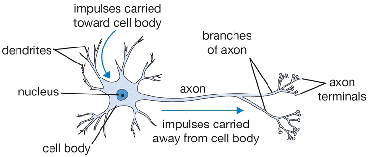
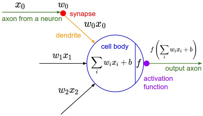A cartoon drawing of a biological neuron (left) and its mathematical model (right).

생물학적 뉴런을 그린 만화(왼쪽)와 그것의 수학적 모델(오른쪽).

An example code for forward-propagating a single neuron might look as follows:

뉴런 하나를 순전파하는 예제 코드는 다음과 같이 생겼을 것이다.

class Neuron(object):
  # ... 
  def forward(self, inputs):
    """ assume inputs and weights are 1-D numpy arrays and bias is a number """
    cell_body_sum = np.sum(inputs * self.weights) + self.bias
    firing_rate = 1.0 / (1.0 + math.exp(-cell_body_sum)) # sigmoid activation function
    return firing_rate

In other words, each neuron performs a dot product with the input and its weights, adds the bias and applies the non-linearity (or activation function), in this case the sigmoid \(\sigma(x) = 1/(1+e^{-x})\). We will go into more details about different activation functions at the end of this section.

다시 말해 각 뉴런은 입력과 자기 가중치의 내적을 구하고 편향을 더한 다음 비선형성(즉 활성화 함수)을 씌운다. 여기서는 sigmoid \(\sigma(x) = 1/(1+e^{-x})\)다. 서로 다른 활성화 함수들은 이 절 끝에서 더 자세히 다룬다.

Coarse model. It’s important to stress that this model of a biological neuron is very coarse: For example, there are many different types of neurons, each with different properties. The dendrites in biological neurons perform complex nonlinear computations. The synapses are not just a single weight, they’re a complex non-linear dynamical system. The exact timing of the output spikes in many systems is known to be important, suggesting that the rate code approximation may not hold. Due to all these and many other simplifications, be prepared to hear groaning sounds from anyone with some neuroscience background if you draw analogies between Neural Networks and real brains. See this review (pdf), or more recently this review if you are interested.

엉성한 모델. 이 생물학적 뉴런 모델이 매우 엉성하다는 점은 짚어둘 필요가 있다. 예를 들어 뉴런에는 성질이 제각각인 종류가 아주 많다. 생물학적 뉴런의 수상돌기는 복잡한 비선형 계산을 수행한다. 시냅스는 가중치 하나가 아니라 복잡한 비선형 동역학계다. 게다가 많은 시스템에서 출력 스파이크가 정확히 언제 나오는지가 중요하다고 알려져 있는데, 이는 발화율 근사가 성립하지 않을 수도 있다는 뜻이다. 이런 것들을 비롯한 수많은 단순화 때문에, 신경망을 진짜 뇌에 빗대어 이야기했다가는 신경과학을 좀 아는 사람이 앓는 소리를 내는 것을 듣게 될 각오를 해야 한다. 관심이 있다면 이 리뷰(pdf)나 더 최근의 이 리뷰를 보라.

Single neuron as a linear classifier

The mathematical form of the model Neuron’s forward computation might look familiar to you. As we saw with linear classifiers, a neuron has the capacity to “like” (activation near one) or “dislike” (activation near zero) certain linear regions of its input space. Hence, with an appropriate loss function on the neuron’s output, we can turn a single neuron into a linear classifier:

모델 뉴런의 순전파 계산이 갖는 수학적 형태가 익숙해 보일 것이다. 선형 분류기에서 봤듯 뉴런도 자기 입력 공간의 특정 선형 영역을 “좋아하거나”(활성값이 1에 가깝다) “싫어할”(활성값이 0에 가깝다) 수 있다. 따라서 뉴런의 출력에 적절한 손실 함수를 붙이면 뉴런 하나를 선형 분류기로 만들 수 있다.

Binary Softmax classifier. For example, we can interpret \(\sigma(\sum_iw_ix_i + b)\) to be the probability of one of the classes \(P(y_i = 1 \mid x_i; w)\). The probability of the other class would be \(P(y_i = 0 \mid x_i; w) = 1 - P(y_i = 1 \mid x_i; w)\), since they must sum to one. With this interpretation, we can formulate the cross-entropy loss as we have seen in the Linear Classification section, and optimizing it would lead to a binary Softmax classifier (also known as logistic regression). Since the sigmoid function is restricted to be between 0-1, the predictions of this classifier are based on whether the output of the neuron is greater than 0.5.

이진 Softmax 분류기. 예를 들어 \(\sigma(\sum_iw_ix_i + b)\)를 두 클래스 중 하나일 확률 \(P(y_i = 1 \mid x_i; w)\)로 해석할 수 있다. 두 확률의 합이 1이어야 하므로 다른 클래스일 확률은 \(P(y_i = 0 \mid x_i; w) = 1 - P(y_i = 1 \mid x_i; w)\)가 된다. 이렇게 해석하면 선형 분류 절에서 본 교차 엔트로피 손실을 세울 수 있고, 그것을 최적화하면 이진 Softmax 분류기(로지스틱 회귀라고도 한다)가 된다. sigmoid 함수의 값은 0에서 1 사이로 제한되어 있으므로 이 분류기의 예측은 뉴런의 출력이 0.5보다 큰지로 갈린다.

Binary SVM classifier. Alternatively, we could attach a max-margin hinge loss to the output of the neuron and train it to become a binary Support Vector Machine.

이진 SVM 분류기. 아니면 뉴런의 출력에 max-margin hinge loss를 붙여 이진 서포트 벡터 머신이 되도록 학습시킬 수도 있다.

Regularization interpretation. The regularization loss in both SVM/Softmax cases could in this biological view be interpreted as gradual forgetting, since it would have the effect of driving all synaptic weights \(w\) towards zero after every parameter update.

정규화의 해석. SVM이든 Softmax든 정규화 손실은 이 생물학적 관점에서 점진적 망각으로 해석할 수 있다. 매개변수를 갱신할 때마다 모든 시냅스 가중치 \(w\)를 0 쪽으로 밀어내는 효과를 내기 때문이다.

역주. L2 정규화 손실 \(\frac{1}{2}\lambda w^2\)의 기울기는 \(\lambda w\)이므로, 갱신 한 번은 \(w \leftarrow w - \eta \lambda w = (1 - \eta\lambda) w\)가 된다. 데이터 손실이 그 가중치를 붙잡아두지 않는 한 갱신할 때마다 가중치에 1보다 작은 수가 곱해져 지수적으로 0에 가까워진다는 뜻이고, 그래서 ‘점진적 망각’이라는 비유가 성립한다. 정규화를 가중치 감쇠(weight decay)라고도 부르는 이유가 이것이다.

A single neuron can be used to implement a binary classifier (e.g. binary Softmax or binary SVM classifiers)

뉴런 하나로 이진 분류기(예컨대 이진 Softmax 분류기나 이진 SVM 분류기)를 구현할 수 있다.

Commonly used activation functions

Every activation function (or non-linearity) takes a single number and performs a certain fixed mathematical operation on it. There are several activation functions you may encounter in practice:

활성화 함수(또는 비선형성)는 하나같이 숫자 하나를 받아 거기에 정해진 수학 연산을 수행한다. 실전에서 마주칠 만한 활성화 함수가 몇 가지 있다.

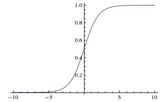
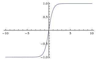Left: Sigmoid non-linearity squashes real numbers to range between [0,1] Right: The tanh non-linearity squashes real numbers to range between [-1,1].

왼쪽: sigmoid 비선형성은 실수를 [0,1] 범위로 눌러 넣는다. 오른쪽: tanh 비선형성은 실수를 [-1,1] 범위로 눌러 넣는다.

Sigmoid. The sigmoid non-linearity has the mathematical form \(\sigma(x) = 1 / (1 + e^{-x})\) and is shown in the image above on the left. As alluded to in the previous section, it takes a real-valued number and “squashes” it into range between 0 and 1. In particular, large negative numbers become 0 and large positive numbers become 1. The sigmoid function has seen frequent use historically since it has a nice interpretation as the firing rate of a neuron: from not firing at all (0) to fully-saturated firing at an assumed maximum frequency (1). In practice, the sigmoid non-linearity has recently fallen out of favor and it is rarely ever used. It has two major drawbacks:

Sigmoid. sigmoid 비선형성은 \(\sigma(x) = 1 / (1 + e^{-x})\)라는 수학적 형태를 가지며 위 그림의 왼쪽에 그려져 있다. 앞 절에서 언급했듯 실숫값 하나를 받아 0과 1 사이로 “눌러 넣는다”. 특히 큰 음수는 0이 되고 큰 양수는 1이 된다. sigmoid 함수는 역사적으로 자주 쓰였다. 뉴런의 발화율로 해석하기 좋기 때문이다. 전혀 발화하지 않는 상태(0)에서 가정된 최대 빈도로 완전히 포화하여 발화하는 상태(1)까지를 나타낸다. 하지만 실전에서 sigmoid 비선형성은 최근 들어 인기를 잃어 이제는 거의 쓰이지 않는다. 큰 단점이 둘 있다.

• Sigmoids saturate and kill gradients. A very undesirable property of the sigmoid neuron is that when the neuron’s activation saturates at either tail of 0 or 1, the gradient at these regions is almost zero. Recall that during backpropagation, this (local) gradient will be multiplied to the gradient of this gate’s output for the whole objective. Therefore, if the local gradient is very small, it will effectively “kill” the gradient and almost no signal will flow through the neuron to its weights and recursively to its data. Additionally, one must pay extra caution when initializing the weights of sigmoid neurons to prevent saturation. For example, if the initial weights are too large then most neurons would become saturated and the network will barely learn.
• Sigmoid outputs are not zero-centered. This is undesirable since neurons in later layers of processing in a Neural Network (more on this soon) would be receiving data that is not zero-centered. This has implications on the dynamics during gradient descent, because if the data coming into a neuron is always positive (e.g. \(x > 0\) elementwise in \(f = w^Tx + b\))), then the gradient on the weights \(w\) will during backpropagation become either all be positive, or all negative (depending on the gradient of the whole expression \(f\)). This could introduce undesirable zig-zagging dynamics in the gradient updates for the weights. However, notice that once these gradients are added up across a batch of data the final update for the weights can have variable signs, somewhat mitigating this issue. Therefore, this is an inconvenience but it has less severe consequences compared to the saturated activation problem above.

• sigmoid는 포화하면서 기울기를 죽인다. sigmoid 뉴런의 아주 바람직하지 않은 성질은, 뉴런의 활성값이 0쪽 꼬리나 1쪽 꼬리에서 포화하면 그 구간의 기울기가 거의 0이 된다는 것이다. 역전파 때 이 (국소) 기울기가 목적 함수 전체에 대한 이 게이트 출력의 기울기와 곱해진다는 점을 떠올려보자. 그러므로 국소 기울기가 아주 작으면 기울기를 사실상 “죽여버려서”, 뉴런을 지나 그 가중치로, 나아가 재귀적으로 그 데이터로 흘러가는 신호가 거의 남지 않는다. 게다가 sigmoid 뉴런의 가중치를 초기화할 때는 포화를 막기 위해 각별히 조심해야 한다. 예컨대 초기 가중치가 너무 크면 대부분의 뉴런이 포화해버려 신경망이 거의 학습하지 못한다.
• sigmoid의 출력은 0을 중심으로 놓이지 않는다. 이는 바람직하지 않다. 신경망에서 뒤쪽 층에 있는 뉴런들이(곧 자세히 다룬다) 0을 중심으로 하지 않는 데이터를 받게 되기 때문이다. 이는 경사 하강법의 동역학에 영향을 준다. 뉴런으로 들어오는 데이터가 항상 양수이면(예컨대 \(f = w^Tx + b\)에서 원소별로 \(x > 0\)이면) 역전파 때 가중치 \(w\)에 대한 기울기가 (식 전체 \(f\)의 기울기에 따라) 전부 양수이거나 전부 음수가 되기 때문이다. 그러면 가중치를 갱신할 때 바람직하지 않은 지그재그 동역학이 생길 수 있다. 다만 데이터 배치 하나에 걸쳐 이 기울기들을 다 더하고 나면 가중치의 최종 갱신량은 부호가 섞일 수 있어서 이 문제가 어느 정도 완화된다는 점에 유의하자. 그러므로 이것은 불편한 점이기는 해도 위의 활성값 포화 문제에 비하면 여파가 덜 심각하다.

역주. 두 번째 단점의 ‘지그재그’는 부호를 따져보면 곧바로 보인다. 뉴런이 \(f = w^Tx + b\)를 계산할 때 가중치 하나에 대한 기울기는 연쇄 법칙으로

\[\frac{\partial L}{\partial w_i} = \frac{\partial L}{\partial f} \, x_i\]

가 된다. 여기서 \(\frac{\partial L}{\partial f}\)는 가중치마다 달라지지 않는 스칼라 하나이므로, 앞 층이 sigmoid라 모든 \(x_i\)가 양수이면 \(\partial L / \partial w_i\)의 부호는 \(i\)와 상관없이 전부 같아진다. 즉 갱신 벡터가 ‘전부 증가’ 아니면 ‘전부 감소’ 두 방향으로만 나올 수 있어서, 어떤 가중치는 올리고 어떤 가중치는 내려야 하는 지점으로 가려면 두 방향을 번갈아 밟는 지그재그 경로를 그릴 수밖에 없다. 원문이 곧이어 말하듯 배치 안에서 여러 예제의 기울기를 더하면 부호가 섞이므로 이 효과는 상당히 누그러진다.

Tanh. The tanh non-linearity is shown on the image above on the right. It squashes a real-valued number to the range [-1, 1]. Like the sigmoid neuron, its activations saturate, but unlike the sigmoid neuron its output is zero-centered. Therefore, in practice the tanh non-linearity is always preferred to the sigmoid nonlinearity. Also note that the tanh neuron is simply a scaled sigmoid neuron, in particular the following holds: \(\tanh(x) = 2 \sigma(2x) -1\).

Tanh. tanh 비선형성은 위 그림의 오른쪽에 그려져 있다. 실숫값을 [-1, 1] 범위로 눌러 넣는다. sigmoid 뉴런처럼 활성값이 포화하지만, sigmoid 뉴런과 달리 출력이 0을 중심으로 놓인다. 그래서 실전에서는 tanh 비선형성이 sigmoid 비선형성보다 언제나 낫다. 또한 tanh 뉴런이 sigmoid 뉴런을 크기 조정한 것에 지나지 않는다는 점에도 유의하자. 구체적으로 \(\tanh(x) = 2 \sigma(2x) -1\)가 성립한다.

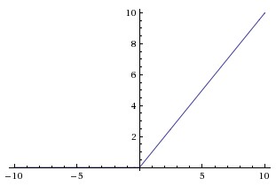
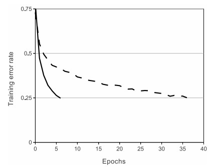Left: Rectified Linear Unit (ReLU) activation function, which is zero when x < 0 and then linear with slope 1 when x > 0. Right: A plot from Krizhevsky et al. (pdf) paper indicating the 6x improvement in convergence with the ReLU unit compared to the tanh unit.

왼쪽: ReLU(Rectified Linear Unit) 활성화 함수. x < 0에서는 0이고 x > 0에서는 기울기(slope)가 1인 직선이다. 오른쪽: Krizhevsky 등(pdf)의 논문에 실린 그래프로, tanh 유닛에 비해 ReLU 유닛의 수렴이 6배 빨라짐을 보여준다.

ReLU. The Rectified Linear Unit has become very popular in the last few years. It computes the function \(f(x) = \max(0, x)\). In other words, the activation is simply thresholded at zero (see image above on the left). There are several pros and cons to using the ReLUs:

ReLU. Rectified Linear Unit은 최근 몇 년 사이 아주 널리 쓰이게 되었다. \(f(x) = \max(0, x)\) 함수를 계산한다. 다시 말해 활성값을 0에서 잘라내기만 한다(위 그림의 왼쪽 참고). ReLU를 쓰는 데는 장점도 단점도 있다.

• (+) It was found to greatly accelerate (e.g. a factor of 6 in Krizhevsky et al.) the convergence of stochastic gradient descent compared to the sigmoid/tanh functions. It is argued that this is due to its linear, non-saturating form.
• (+) Compared to tanh/sigmoid neurons that involve expensive operations (exponentials, etc.), the ReLU can be implemented by simply thresholding a matrix of activations at zero.
• (-) Unfortunately, ReLU units can be fragile during training and can “die”. For example, a large gradient flowing through a ReLU neuron could cause the weights to update in such a way that the neuron will never activate on any datapoint again. If this happens, then the gradient flowing through the unit will forever be zero from that point on. That is, the ReLU units can irreversibly die during training since they can get knocked off the data manifold. For example, you may find that as much as 40% of your network can be “dead” (i.e. neurons that never activate across the entire training dataset) if the learning rate is set too high. With a proper setting of the learning rate this is less frequently an issue.

• (+) sigmoid/tanh 함수에 비해 SGD의 수렴을 크게 가속하는 것으로 밝혀졌다(예컨대 Krizhevsky 등에서는 6배). 선형이고 포화하지 않는 형태 덕분이라고 이야기된다.
• (+) 지수 함수 같은 비싼 연산이 들어가는 tanh/sigmoid 뉴런과 달리, ReLU는 활성값 행렬을 0에서 잘라내기만 하면 구현된다.
• (-) 안타깝게도 ReLU 유닛은 학습 도중 망가지기 쉽고 “죽어버릴” 수 있다. 예를 들어 큰 기울기가 ReLU 뉴런을 지나가면서 가중치가 갱신된 결과, 그 뉴런이 어떤 데이터 점에 대해서도 두 번 다시 활성화되지 않게 될 수 있다. 이렇게 되면 그 시점부터 그 유닛을 지나는 기울기는 영원히 0이 된다. 즉 ReLU 유닛은 데이터 다양체(data manifold) 바깥으로 밀려날 수 있어서 학습 중에 돌이킬 수 없이 죽어버릴 수 있다. 예컨대 학습률을 너무 높게 잡으면 신경망의 40%나 되는 부분이 “죽어 있는”(즉 학습 데이터셋 전체에 걸쳐 한 번도 활성화되지 않는) 것을 보게 될 수도 있다. 학습률을 적절히 잡으면 이 문제는 덜 자주 나타난다.

역주. sigmoid의 포화와 ReLU의 죽음은 겉보기에 비슷하지만 결정적으로 다르다. 포화한 sigmoid의 기울기는 아주 작을 뿐 0이 아니어서, 들어오는 입력이 달라지면 뉴런이 다시 살아날 여지가 남는다. 반면 ReLU는 \(w^Tx + b < 0\)인 구간에서 기울기가 정확히 0이다. 어떤 뉴런의 편향이 크게 음수 쪽으로 밀려나 학습 데이터 전체에 대해 입력의 합이 음수가 되어버리면, 그 뉴런으로 들어오는 기울기는 모든 예제에서 0이 되고 가중치도 편향도 다시는 갱신되지 않는다. 되살릴 방법이 없다는 뜻이며, 원문이 ‘돌이킬 수 없이 죽는다’고 쓴 이유가 이것이다. 아래 보충에서 학습률을 올려가며 실제로 세어본다.

Leaky ReLU. Leaky ReLUs are one attempt to fix the “dying ReLU” problem. Instead of the function being zero when x < 0, a leaky ReLU will instead have a small positive slope (of 0.01, or so). That is, the function computes \(f(x) = \mathbb{1}(x < 0) (\alpha x) + \mathbb{1}(x>=0) (x)\) where \(\alpha\) is a small constant. Some people report success with this form of activation function, but the results are not always consistent. The slope in the negative region can also be made into a parameter of each neuron, as seen in PReLU neurons, introduced in Delving Deep into Rectifiers, by Kaiming He et al., 2015. However, the consistency of the benefit across tasks is presently unclear.

Leaky ReLU. Leaky ReLU는 “죽는 ReLU” 문제를 고쳐보려는 시도 중 하나다. x < 0에서 함수를 0으로 두는 대신 작은 양의 기울기(slope)를 준다(0.01 정도). 즉 \(f(x) = \mathbb{1}(x < 0) (\alpha x) + \mathbb{1}(x>=0) (x)\)를 계산하며 \(\alpha\)는 작은 상수다. 이 형태의 활성화 함수로 재미를 봤다는 보고가 있기는 하지만 결과가 늘 일관되지는 않다. 음수 구간의 기울기(slope)를 뉴런마다의 매개변수로 만들 수도 있는데, Kaiming He 등이 2015년 Delving Deep into Rectifiers에서 소개한 PReLU 뉴런이 그렇다. 다만 그 이득이 과제를 가리지 않고 일관되게 나타나는지는 현재로선 분명치 않다.

Maxout. Other types of units have been proposed that do not have the functional form \(f(w^Tx + b)\) where a non-linearity is applied on the dot product between the weights and the data. One relatively popular choice is the Maxout neuron (introduced recently by Goodfellow et al.) that generalizes the ReLU and its leaky version. The Maxout neuron computes the function \(\max(w_1^Tx+b_1, w_2^Tx + b_2)\). Notice that both ReLU and Leaky ReLU are a special case of this form (for example, for ReLU we have \(w_1, b_1 = 0\)). The Maxout neuron therefore enjoys all the benefits of a ReLU unit (linear regime of operation, no saturation) and does not have its drawbacks (dying ReLU). However, unlike the ReLU neurons it doubles the number of parameters for every single neuron, leading to a high total number of parameters.

Maxout. 가중치와 데이터의 내적에 비선형성을 씌우는 \(f(w^Tx + b)\) 형태가 아닌 다른 종류의 유닛들도 제안되었다. 비교적 널리 쓰이는 것이 Goodfellow 등이 최근 소개한 Maxout 뉴런으로, ReLU와 그 leaky 버전을 일반화한다. Maxout 뉴런은 \(\max(w_1^Tx+b_1, w_2^Tx + b_2)\) 함수를 계산한다. ReLU와 Leaky ReLU 모두 이 형태의 특수한 경우라는 점에 주목하자(예컨대 ReLU는 \(w_1, b_1 = 0\)인 경우다). 따라서 Maxout 뉴런은 ReLU 유닛의 장점(선형 구간에서 동작하고 포화하지 않는다)을 전부 누리면서 그 단점(죽는 ReLU)은 없다. 다만 ReLU 뉴런과 달리 뉴런 하나마다 매개변수가 두 배로 늘어나므로 전체 매개변수 수가 많아진다.

This concludes our discussion of the most common types of neurons and their activation functions. As a last comment, it is very rare to mix and match different types of neurons in the same network, even though there is no fundamental problem with doing so.

여기까지가 가장 흔한 뉴런 종류와 그 활성화 함수에 대한 이야기다. 마지막으로 덧붙이자면, 한 신경망 안에서 서로 다른 종류의 뉴런을 섞어 쓰는 일은 원리상 아무 문제가 없는데도 아주 드물다.

TLDR: “What neuron type should I use?” Use the ReLU non-linearity, be careful with your learning rates and possibly monitor the fraction of “dead” units in a network. If this concerns you, give Leaky ReLU or Maxout a try. Never use sigmoid. Try tanh, but expect it to work worse than ReLU/Maxout.

TLDR: “어떤 뉴런을 써야 하나?” ReLU 비선형성을 쓰되 학습률에 조심하고, 가능하면 신경망에서 “죽은” 유닛의 비율을 지켜보라. 그것이 걱정된다면 Leaky ReLU나 Maxout을 시도해보라. sigmoid는 절대 쓰지 마라. tanh는 시도해봐도 좋지만 ReLU/Maxout보다는 못할 것이라고 예상하라.

역주. ‘sigmoid는 절대 쓰지 마라’는 조언은 은닉층의 활성화 함수를 두고 하는 말이다. 출력층에서 확률을 내놓아야 하는 자리(이진 분류의 출력)나 LSTM의 게이트처럼 0과 1 사이의 여닫이 값이 필요한 자리에서는 sigmoid가 지금도 표준이다. 이 절이 문제 삼는 것은 신호를 층층이 통과시켜야 하는 은닉 유닛에서 sigmoid가 기울기를 죽인다는 점이지, 함수 자체가 쓸모없다는 것이 아니다.

보충: 학습률을 올리면 정말로 뉴런이 죽는지 세어보기

원문은 “학습률을 너무 높게 잡으면 신경망의 40%나 되는 부분이 죽어 있는 것을 보게 될 수도 있다”고만 말하고 넘어간다. 은닉 뉴런 100개짜리 2층 신경망을 XOR 모양의 장난감 데이터에 학습시킨 다음, 학습 데이터 300개 전부에 대해 한 번도 켜지지 않은 ReLU가 몇 개인지 직접 세어보자.

import numpy as np

np.random.seed(0)
N, D, H = 300, 2, 100                        # 예제 300개, 입력 2차원, 은닉 뉴런 100개
X = np.random.randn(N, D)
y = (X[:, 0] * X[:, 1] > 0).astype(int)      # XOR 모양이라 은닉층이 반드시 필요하다

def train(lr, steps=200):
    rng = np.random.RandomState(1)
    W1, b1 = 0.1 * rng.randn(D, H), np.zeros(H)
    W2, b2 = 0.1 * rng.randn(H, 2), np.zeros(2)
    for _ in range(steps):
        h = np.maximum(0, X.dot(W1) + b1)                    # ReLU
        scores = h.dot(W2) + b2
        p = np.exp(scores - scores.max(1, keepdims=True))
        p /= p.sum(1, keepdims=True)
        dscores = p.copy()
        dscores[range(N), y] -= 1
        dscores /= N
        dW2, db2 = h.T.dot(dscores), dscores.sum(0)
        dh = dscores.dot(W2.T)
        dh[h <= 0] = 0                                       # ReLU 게이트를 통과하는 기울기
        dW1, db1 = X.T.dot(dh), dh.sum(0)
        for param, grad in ((W1, dW1), (b1, db1), (W2, dW2), (b2, db2)):
            param -= lr * grad
    h = np.maximum(0, X.dot(W1) + b1)
    dead = int((h.max(0) == 0).sum())        # 학습 데이터 전체에서 한 번도 켜지지 않은 뉴런
    scores = h.dot(W2) + b2
    p = np.exp(scores - scores.max(1, keepdims=True))
    p /= p.sum(1, keepdims=True)
    return dead, -np.log(p[range(N), y]).mean()

for lr in (0.1, 1.0, 10.0, 50.0):
    dead, loss = train(lr)
    print("학습률 %5.1f  ->  죽은 ReLU %3d/100개,  손실 %.4f" % (lr, dead, loss))

학습률   0.1  ->  죽은 ReLU   0/100개,  손실 0.2471
학습률   1.0  ->  죽은 ReLU   0/100개,  손실 0.0504
학습률  10.0  ->  죽은 ReLU  90/100개,  손실 1.4446
학습률  50.0  ->  죽은 ReLU  99/100개,  손실 8.7692

학습률 1.0까지는 죽은 뉴런이 하나도 없고 손실도 잘 내려간다. 10.0에서는 은닉 뉴런 100개 중 90개가 학습 데이터 전체에 대해 음수 구간으로 밀려나 죽어버리고, 남은 10개만으로 버티느라 손실이 무작위 추측(약 0.69)보다도 나빠진다. 50.0에서는 99개가 죽는다. 바꾼 것은 학습률 하나뿐인데 신경망의 대부분이 영구히 사라진 셈이다.

Neural Network architectures

Layer-wise organization

Neural Networks as neurons in graphs. Neural Networks are modeled as collections of neurons that are connected in an acyclic graph. In other words, the outputs of some neurons can become inputs to other neurons. Cycles are not allowed since that would imply an infinite loop in the forward pass of a network. Instead of an amorphous blobs of connected neurons, Neural Network models are often organized into distinct layers of neurons. For regular neural networks, the most common layer type is the fully-connected layer in which neurons between two adjacent layers are fully pairwise connected, but neurons within a single layer share no connections. Below are two example Neural Network topologies that use a stack of fully-connected layers:

그래프 위의 뉴런으로 본 신경망. 신경망은 비순환 그래프로 연결된 뉴런들의 모음으로 모델링한다. 다시 말해 어떤 뉴런의 출력이 다른 뉴런의 입력이 될 수 있다. 순환은 허용되지 않는데, 순환이 있으면 신경망의 순전파가 무한 루프에 빠진다는 뜻이 되기 때문이다. 신경망 모델은 뉴런들이 아무렇게나 뭉친 덩어리 대신 뚜렷이 구분되는 층으로 구성되는 경우가 많다. 보통의 신경망에서 가장 흔한 층 유형은 완전 연결 층(fully-connected layer)이다. 이웃한 두 층 사이의 뉴런은 쌍마다 빠짐없이 연결되지만 같은 층 안의 뉴런끼리는 연결이 없는 층이다. 아래는 완전 연결 층을 쌓아 만든 신경망 위상 구조 두 가지 예다.

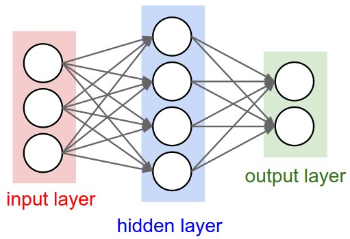
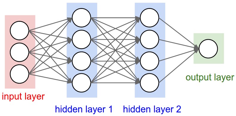Left: A 2-layer Neural Network (one hidden layer of 4 neurons (or units) and one output layer with 2 neurons), and three inputs. Right: A 3-layer neural network with three inputs, two hidden layers of 4 neurons each and one output layer. Notice that in both cases there are connections (synapses) between neurons across layers, but not within a layer.

왼쪽: 2층 신경망(뉴런 또는 유닛 4개짜리 은닉층 하나와 뉴런 2개짜리 출력층 하나)이며 입력은 3개다. 오른쪽: 입력 3개, 각각 뉴런 4개짜리 은닉층 둘, 출력층 하나로 이루어진 3층 신경망. 두 경우 모두 층을 가로지르는 뉴런들 사이에는 연결(시냅스)이 있지만 한 층 안에서는 없다는 점에 주목하자.

Naming conventions. Notice that when we say N-layer neural network, we do not count the input layer. Therefore, a single-layer neural network describes a network with no hidden layers (input directly mapped to output). In that sense, you can sometimes hear people say that logistic regression or SVMs are simply a special case of single-layer Neural Networks. You may also hear these networks interchangeably referred to as “Artificial Neural Networks” (ANN) or “Multi-Layer Perceptrons” (MLP). Many people do not like the analogies between Neural Networks and real brains and prefer to refer to neurons as units.

이름 붙이는 관례. N층 신경망이라고 할 때 입력층은 세지 않는다는 점에 주의하자. 따라서 1층 신경망이란 은닉층이 없는 신경망, 즉 입력이 곧바로 출력으로 이어지는 신경망을 가리킨다. 그런 뜻에서 로지스틱 회귀나 SVM이 1층 신경망의 특수한 경우일 뿐이라고 말하는 것을 가끔 들을 수 있다. 이런 신경망을 “인공 신경망(Artificial Neural Networks, ANN)”이나 “다층 퍼셉트론(Multi-Layer Perceptrons, MLP)”이라고 부르는 것도 볼 수 있다. 신경망을 진짜 뇌에 빗대는 것을 싫어해서 뉴런 대신 유닛(unit)이라고 부르기를 선호하는 사람도 많다.

Output layer. Unlike all layers in a Neural Network, the output layer neurons most commonly do not have an activation function (or you can think of them as having a linear identity activation function). This is because the last output layer is usually taken to represent the class scores (e.g. in classification), which are arbitrary real-valued numbers, or some kind of real-valued target (e.g. in regression).

출력층. 신경망의 다른 모든 층과 달리 출력층 뉴런에는 활성화 함수가 없는 것이 가장 흔하다(항등 함수를 활성화 함수로 갖는다고 생각해도 된다). 마지막 출력층은 보통 (분류에서라면) 임의의 실숫값인 클래스 점수를 나타내거나 (회귀에서라면) 어떤 실숫값 목표치를 나타내는 것으로 보기 때문이다.

Sizing neural networks. The two metrics that people commonly use to measure the size of neural networks are the number of neurons, or more commonly the number of parameters. Working with the two example networks in the above picture:

신경망의 크기 재기. 신경망의 크기를 재는 데 흔히 쓰는 지표는 뉴런의 개수, 또는 더 흔하게는 매개변수의 개수 둘이다. 위 그림의 신경망 두 개를 예로 들어보자.

• The first network (left) has 4 + 2 = 6 neurons (not counting the inputs), [3 x 4] + [4 x 2] = 20 weights and 4 + 2 = 6 biases, for a total of 26 learnable parameters.
• The second network (right) has 4 + 4 + 1 = 9 neurons, [3 x 4] + [4 x 4] + [4 x 1] = 12 + 16 + 4 = 32 weights and 4 + 4 + 1 = 9 biases, for a total of 41 learnable parameters.

• 첫 번째 신경망(왼쪽)은 뉴런이 4 + 2 = 6개(입력은 세지 않는다), 가중치가 [3 x 4] + [4 x 2] = 20개, 편향이 4 + 2 = 6개이므로, 학습되는 매개변수가 모두 26개다.
• 두 번째 신경망(오른쪽)은 뉴런이 4 + 4 + 1 = 9개, 가중치가 [3 x 4] + [4 x 4] + [4 x 1] = 12 + 16 + 4 = 32개, 편향이 4 + 4 + 1 = 9개이므로, 학습되는 매개변수가 모두 41개다.

To give you some context, modern Convolutional Networks contain on orders of 100 million parameters and are usually made up of approximately 10-20 layers (hence deep learning). However, as we will see the number of effective connections is significantly greater due to parameter sharing. More on this in the Convolutional Neural Networks module.

감을 잡을 수 있도록 덧붙이면, 요즘의 합성곱 신경망은 매개변수가 1억 개 규모이고 보통 10~20개 층으로 이루어진다(그래서 딥러닝이다). 다만 뒤에서 보겠지만 매개변수 공유 덕분에 실효 연결 수는 그보다 훨씬 많다. 이에 대해서는 합성곱 신경망 모듈에서 더 다룬다.

Example feed-forward computation

Repeated matrix multiplications interwoven with activation function. One of the primary reasons that Neural Networks are organized into layers is that this structure makes it very simple and efficient to evaluate Neural Networks using matrix vector operations. Working with the example three-layer neural network in the diagram above, the input would be a [3x1] vector. All connection strengths for a layer can be stored in a single matrix. For example, the first hidden layer’s weights W1 would be of size [4x3], and the biases for all units would be in the vector b1, of size [4x1]. Here, every single neuron has its weights in a row of W1, so the matrix vector multiplication np.dot(W1,x) evaluates the activations of all neurons in that layer. Similarly, W2 would be a [4x4] matrix that stores the connections of the second hidden layer, and W3 a [1x4] matrix for the last (output) layer. The full forward pass of this 3-layer neural network is then simply three matrix multiplications, interwoven with the application of the activation function:

활성화 함수와 번갈아 반복되는 행렬 곱. 신경망을 층으로 구성하는 주된 이유 중 하나는, 이 구조 덕분에 행렬-벡터 연산으로 신경망을 아주 간단하고 효율적으로 평가할 수 있다는 것이다. 위 그림의 3층 신경망 예제로 이야기하면 입력은 [3x1] 벡터다. 한 층의 모든 연결 세기는 행렬 하나에 담을 수 있다. 예를 들어 첫 은닉층의 가중치 W1은 [4x3] 크기가 되고 모든 유닛의 편향은 [4x1] 크기의 벡터 b1에 담긴다. 여기서 뉴런 하나하나의 가중치는 W1의 한 행에 들어 있으므로, 행렬-벡터 곱 np.dot(W1,x)가 그 층에 있는 모든 뉴런의 활성값을 한꺼번에 계산한다. 마찬가지로 W2는 두 번째 은닉층의 연결을 담는 [4x4] 행렬이고 W3는 마지막 (출력)층의 [1x4] 행렬이다. 그러면 이 3층 신경망의 순전파 전체는 활성화 함수 적용과 번갈아 이루어지는 행렬 곱 세 번에 지나지 않는다.

# forward-pass of a 3-layer neural network:
f = lambda x: 1.0/(1.0 + np.exp(-x)) # activation function (use sigmoid)
x = np.random.randn(3, 1) # random input vector of three numbers (3x1)
h1 = f(np.dot(W1, x) + b1) # calculate first hidden layer activations (4x1)
h2 = f(np.dot(W2, h1) + b2) # calculate second hidden layer activations (4x1)
out = np.dot(W3, h2) + b3 # output neuron (1x1)

In the above code, W1,W2,W3,b1,b2,b3 are the learnable parameters of the network. Notice also that instead of having a single input column vector, the variable x could hold an entire batch of training data (where each input example would be a column of x) and then all examples would be efficiently evaluated in parallel. Notice that the final Neural Network layer usually doesn’t have an activation function (e.g. it represents a (real-valued) class score in a classification setting).

위 코드에서 W1,W2,W3,b1,b2,b3는 신경망의 학습되는 매개변수다. 또한 입력 열벡터 하나만 두는 대신 변수 x가 학습 데이터 배치 전체를 담을 수도 있고(각 입력 예제가 x의 한 열이 된다) 그러면 모든 예제를 병렬로 효율적으로 평가할 수 있다는 점에도 주목하자. 신경망의 마지막 층에는 보통 활성화 함수가 없다는 점에도 유의하자(예컨대 분류 상황에서는 (실숫값) 클래스 점수를 나타낸다).

The forward pass of a fully-connected layer corresponds to one matrix multiplication followed by a bias offset and an activation function.

완전 연결 층의 순전파는 행렬 곱 한 번에 편향을 더하고 활성화 함수를 씌우는 것에 해당한다.

Representational power

One way to look at Neural Networks with fully-connected layers is that they define a family of functions that are parameterized by the weights of the network. A natural question that arises is: What is the representational power of this family of functions? In particular, are there functions that cannot be modeled with a Neural Network?

완전 연결 층으로 이루어진 신경망을 보는 한 가지 관점은, 신경망이 자기 가중치로 매개변수화된 함수족을 정의한다고 보는 것이다. 그러면 자연스럽게 이런 질문이 떠오른다. 이 함수족의 표현력(representational power)은 어느 정도인가? 특히, 신경망으로 모델링할 수 없는 함수가 있는가?

It turns out that Neural Networks with at least one hidden layer are universal approximators. That is, it can be shown (e.g. see Approximation by Superpositions of Sigmoidal Function from 1989 (pdf), or this intuitive explanation from Michael Nielsen) that given any continuous function \(f(x)\) and some \(\epsilon > 0\), there exists a Neural Network \(g(x)\) with one hidden layer (with a reasonable choice of non-linearity, e.g. sigmoid) such that \(\forall x, \mid f(x) - g(x) \mid < \epsilon\). In other words, the neural network can approximate any continuous function.

은닉층이 하나 이상인 신경망은 보편 근사기(universal approximator)임이 밝혀져 있다. 즉 어떤 연속 함수 \(f(x)\)와 어떤 \(\epsilon > 0\)이 주어지든, 비선형성만 적당히 고르면(예컨대 sigmoid) \(\forall x, \mid f(x) - g(x) \mid < \epsilon\)을 만족하는 은닉층 하나짜리 신경망 \(g(x)\)가 존재함을 보일 수 있다(예컨대 1989년의 Approximation by Superpositions of Sigmoidal Function(pdf)이나 Michael Nielsen의 직관적인 설명을 보라). 다시 말해 신경망은 어떤 연속 함수든 근사할 수 있다.

If one hidden layer suffices to approximate any function, why use more layers and go deeper? The answer is that the fact that a two-layer Neural Network is a universal approximator is, while mathematically cute, a relatively weak and useless statement in practice. In one dimension, the “sum of indicator bumps” function \(g(x) = \sum_i c_i \mathbb{1}(a_i < x < b_i)\) where \(a,b,c\) are parameter vectors is also a universal approximator, but no one would suggest that we use this functional form in Machine Learning. Neural Networks work well in practice because they compactly express nice, smooth functions that fit well with the statistical properties of data we encounter in practice, and are also easy to learn using our optimization algorithms (e.g. gradient descent). Similarly, the fact that deeper networks (with multiple hidden layers) can work better than a single-hidden-layer networks is an empirical observation, despite the fact that their representational power is equal.

은닉층 하나로 어떤 함수든 근사할 수 있다면 왜 층을 더 쌓아 깊이 들어가는가? 답은 이렇다. 2층 신경망이 보편 근사기라는 사실은 수학적으로는 깜찍하지만 실전에서는 상당히 약하고 쓸모없는 진술이다. 1차원에서 “지시 함수 봉우리의 합”인 함수 \(g(x) = \sum_i c_i \mathbb{1}(a_i < x < b_i)\) 역시 보편 근사기다. 여기서 \(a,b,c\)는 매개변수 벡터다. 하지만 이 형태의 함수를 기계 학습에 쓰자고 할 사람은 아무도 없다. 신경망이 실전에서 잘 되는 이유는, 우리가 실제로 마주치는 데이터의 통계적 성질에 잘 들어맞는 매끄럽고 좋은 함수들을 간결하게 표현하면서 동시에 우리가 쓰는 최적화 알고리즘(예컨대 경사 하강법)으로 학습시키기도 쉽기 때문이다. 마찬가지로, 은닉층이 여럿인 더 깊은 신경망이 은닉층 하나짜리 신경망보다 잘 될 수 있다는 것도 — 둘의 표현력이 같은데도 — 경험적인 관찰이다.

As an aside, in practice it is often the case that 3-layer neural networks will outperform 2-layer nets, but going even deeper (4,5,6-layer) rarely helps much more. This is in stark contrast to Convolutional Networks, where depth has been found to be an extremely important component for a good recognition system (e.g. on order of 10 learnable layers). One argument for this observation is that images contain hierarchical structure (e.g. faces are made up of eyes, which are made up of edges, etc.), so several layers of processing make intuitive sense for this data domain.

덧붙이자면 실전에서는 3층 신경망이 2층 신경망보다 나은 경우가 많지만, 거기서 더 깊이 4, 5, 6층으로 들어가는 것은 별 도움이 되지 않는 일이 잦다. 이는 좋은 인식 시스템을 만드는 데 깊이가 극히 중요한 요소임이 밝혀진 합성곱 신경망(예컨대 학습되는 층이 10개 규모다)과 극명하게 대비된다. 이 관찰을 설명하는 한 가지 주장은 이미지가 계층적 구조를 담고 있다는 것이다(예컨대 얼굴은 눈으로 이루어지고 눈은 모서리로 이루어진다). 그러니 이 데이터 영역에서는 여러 층에 걸친 처리가 직관적으로 말이 된다.

The full story is, of course, much more involved and a topic of much recent research. If you are interested in these topics we recommend for further reading:

물론 전체 이야기는 훨씬 복잡하고 최근 연구가 활발한 주제다. 이런 주제에 관심이 있다면 다음 읽을거리를 권한다.

• Deep Learning book in press by Bengio, Goodfellow, Courville, in particular Chapter 6.4.
• Do Deep Nets Really Need to be Deep?
• FitNets: Hints for Thin Deep Nets

• Bengio, Goodfellow, Courville이 쓰고 있는 Deep Learning 책, 특히 6.4장.
• Do Deep Nets Really Need to be Deep?
• FitNets: Hints for Thin Deep Nets

Setting number of layers and their sizes

How do we decide on what architecture to use when faced with a practical problem? Should we use no hidden layers? One hidden layer? Two hidden layers? How large should each layer be? First, note that as we increase the size and number of layers in a Neural Network, the capacity of the network increases. That is, the space of representable functions grows since the neurons can collaborate to express many different functions. For example, suppose we had a binary classification problem in two dimensions. We could train three separate neural networks, each with one hidden layer of some size and obtain the following classifiers:

실제 문제를 마주했을 때 어떤 구조를 쓸지는 어떻게 정할까? 은닉층을 두지 말아야 할까? 하나? 둘? 각 층은 얼마나 커야 할까? 우선, 신경망의 층 크기와 층 수를 늘리면 신경망의 수용력(capacity)이 커진다는 점에 주목하자. 즉 뉴런들이 협력해 여러 다른 함수를 표현할 수 있으므로 표현 가능한 함수의 공간이 넓어진다. 예를 들어 2차원에서 이진 분류 문제가 있다고 하자. 각각 크기가 다른 은닉층 하나씩을 가진 신경망 셋을 따로 학습시켜 다음과 같은 분류기를 얻을 수 있다.

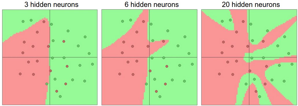Larger Neural Networks can represent more complicated functions. The data are shown as circles colored by their class, and the decision regions by a trained neural network are shown underneath. You can play with these examples in this ConvNetsJS demo.

더 큰 신경망은 더 복잡한 함수를 표현할 수 있다. 데이터는 클래스에 따라 색이 다른 원으로 나타냈고, 학습된 신경망의 결정 영역(decision region)은 그 아래에 나타냈다. 이 예제들은 ConvNetsJS 데모에서 직접 만져볼 수 있다.

In the diagram above, we can see that Neural Networks with more neurons can express more complicated functions. However, this is both a blessing (since we can learn to classify more complicated data) and a curse (since it is easier to overfit the training data). Overfitting occurs when a model with high capacity fits the noise in the data instead of the (assumed) underlying relationship. For example, the model with 20 hidden neurons fits all the training data but at the cost of segmenting the space into many disjoint red and green decision regions. The model with 3 hidden neurons only has the representational power to classify the data in broad strokes. It models the data as two blobs and interprets the few red points inside the green cluster as outliers (noise). In practice, this could lead to better generalization on the test set.

위 그림에서 뉴런이 더 많은 신경망이 더 복잡한 함수를 표현할 수 있음을 볼 수 있다. 그런데 이것은 축복이자(더 복잡한 데이터를 분류하도록 학습할 수 있으므로) 저주다(학습 데이터에 과적합하기가 더 쉬우므로). 과적합은 수용력이 큰 모델이 (있다고 가정한) 밑바탕의 관계 대신 데이터의 잡음에 맞춰질 때 일어난다. 예컨대 은닉 뉴런이 20개인 모델은 학습 데이터 전부에 들어맞지만, 그 대가로 공간을 서로 떨어진 빨강·초록 결정 영역 여럿으로 쪼개놓았다. 은닉 뉴런이 3개인 모델은 데이터를 큰 붓질로 분류할 만큼의 표현력밖에 없다. 이 모델은 데이터를 두 덩어리로 보고 초록 무리 안에 있는 몇 개의 빨간 점을 이상치(잡음)로 해석한다. 실전에서는 이쪽이 테스트 집합에서 더 나은 일반화로 이어질 수 있다.

Based on our discussion above, it seems that smaller neural networks can be preferred if the data is not complex enough to prevent overfitting. However, this is incorrect - there are many other preferred ways to prevent overfitting in Neural Networks that we will discuss later (such as L2 regularization, dropout, input noise). In practice, it is always better to use these methods to control overfitting instead of the number of neurons.

지금까지의 이야기를 보면, 데이터가 그리 복잡하지 않을 때는 과적합을 막기 위해 작은 신경망을 쓰는 편이 낫겠다 싶다. 하지만 그것은 틀렸다. 신경망에서 과적합을 막는 데 더 선호되는 방법이 뒤에서 다룰 것들로 여럿 있다(L2 정규화, dropout, 입력 잡음 등). 실전에서는 과적합을 뉴런 개수로 다스리는 대신 언제나 이런 방법들을 쓰는 편이 낫다.

The subtle reason behind this is that smaller networks are harder to train with local methods such as Gradient Descent: It’s clear that their loss functions have relatively few local minima, but it turns out that many of these minima are easier to converge to, and that they are bad (i.e. with high loss). Conversely, bigger neural networks contain significantly more local minima, but these minima turn out to be much better in terms of their actual loss. Since Neural Networks are non-convex, it is hard to study these properties mathematically, but some attempts to understand these objective functions have been made, e.g. in a recent paper The Loss Surfaces of Multilayer Networks. In practice, what you find is that if you train a small network the final loss can display a good amount of variance - in some cases you get lucky and converge to a good place but in some cases you get trapped in one of the bad minima. On the other hand, if you train a large network you’ll start to find many different solutions, but the variance in the final achieved loss will be much smaller. In other words, all solutions are about equally as good, and rely less on the luck of random initialization.

그 이면의 미묘한 이유는, 작은 신경망이 경사 하강법 같은 국소적 방법으로 학습시키기가 더 어렵다는 데 있다. 작은 신경망의 손실 함수에 국소 최솟값(local minima)이 비교적 적다는 것은 분명하지만, 그중 많은 수가 수렴해 들어가기 쉬운 데다 나쁜(즉 손실이 큰) 최솟값인 것으로 드러난다. 반대로 큰 신경망은 국소 최솟값을 훨씬 많이 품고 있지만, 그 최솟값들은 실제 손실 면에서 훨씬 낫다. 신경망은 볼록하지 않아서 이런 성질을 수학적으로 연구하기가 어렵지만, 이 목적 함수들을 이해하려는 시도가 몇 가지 있었다. 예컨대 최근 논문 The Loss Surfaces of Multilayer Networks가 그렇다. 실제로 해보면, 작은 신경망을 학습시켰을 때 최종 손실의 분산이 꽤 크다는 것을 알게 된다. 운이 좋아 좋은 곳으로 수렴할 때도 있지만 나쁜 최솟값 하나에 갇힐 때도 있다. 반면 큰 신경망을 학습시키면 서로 다른 해를 여럿 찾게 되지만 최종적으로 도달한 손실의 분산은 훨씬 작다. 다시 말해 모든 해가 얼추 비슷하게 좋고, 무작위 초기화의 운에 덜 기댄다.

To reiterate, the regularization strength is the preferred way to control the overfitting of a neural network. We can look at the results achieved by three different settings:

다시 말하지만, 신경망의 과적합을 다스리는 데 선호되는 방법은 정규화 세기다. 서로 다른 세 가지 설정으로 얻은 결과를 보자.

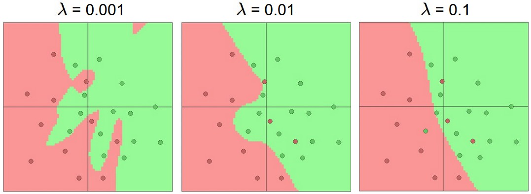The effects of regularization strength: Each neural network above has 20 hidden neurons, but changing the regularization strength makes its final decision regions smoother with a higher regularization. You can play with these examples in this ConvNetsJS demo.

정규화 세기의 효과. 위 신경망은 모두 은닉 뉴런이 20개지만, 정규화 세기를 높이면 최종 결정 영역이 더 매끄러워진다. 이 예제들은 ConvNetsJS 데모에서 직접 만져볼 수 있다.

The takeaway is that you should not be using smaller networks because you are afraid of overfitting. Instead, you should use as big of a neural network as your computational budget allows, and use other regularization techniques to control overfitting.

요점은, 과적합이 두려워서 더 작은 신경망을 써서는 안 된다는 것이다. 대신 계산 예산이 허락하는 한 큰 신경망을 쓰고, 과적합은 다른 정규화 기법으로 다스려야 한다.

Summary

In summary,

정리하면 다음과 같다.

• We introduced a very coarse model of a biological neuron.
• We discussed several types of activation functions that are used in practice, with ReLU being the most common choice.
• We introduced Neural Networks where neurons are connected with Fully-Connected layers where neurons in adjacent layers have full pair-wise connections, but neurons within a layer are not connected.
• We saw that this layered architecture enables very efficient evaluation of Neural Networks based on matrix multiplications interwoven with the application of the activation function.
• We saw that that Neural Networks are universal function approximators, but we also discussed the fact that this property has little to do with their ubiquitous use. They are used because they make certain “right” assumptions about the functional forms of functions that come up in practice.
• We discussed the fact that larger networks will always work better than smaller networks, but their higher model capacity must be appropriately addressed with stronger regularization (such as higher weight decay), or they might overfit. We will see more forms of regularization (especially dropout) in later sections.

• 생물학적 뉴런의 아주 엉성한 모델을 소개했다.
• 실전에서 쓰는 여러 종류의 활성화 함수를 다뤘고, 그중 가장 흔한 선택은 ReLU다.
• 이웃한 층의 뉴런끼리는 쌍마다 빠짐없이 연결되지만 같은 층 안의 뉴런끼리는 연결되지 않는 완전 연결 층으로 뉴런들을 이은 신경망을 소개했다.
• 이 층 구조 덕분에 활성화 함수 적용과 번갈아 이루어지는 행렬 곱으로 신경망을 아주 효율적으로 평가할 수 있음을 봤다.
• 신경망이 보편 함수 근사기임을 봤지만, 이 성질이 신경망이 널리 쓰이는 이유와는 별 상관이 없다는 사실도 이야기했다. 신경망이 쓰이는 이유는 실전에서 마주치는 함수들의 형태에 대해 어떤 “옳은” 가정을 하기 때문이다.
• 큰 신경망은 언제나 작은 신경망보다 잘 되지만, 그만큼 커진 모델 수용력은 더 강한 정규화(예컨대 더 큰 가중치 감쇠)로 적절히 다스려야 하며 그러지 않으면 과적합할 수 있다는 것을 이야기했다. 정규화의 다른 형태들, 특히 dropout은 뒤쪽 절에서 더 본다.

Additional References

• deeplearning.net tutorial with Theano
• ConvNetJS demos for intuitions
• Michael Nielsen’s tutorials

• Theano를 쓰는 deeplearning.net 튜토리얼
• 직관을 얻기 좋은 ConvNetJS 데모
• Michael Nielsen의 튜토리얼