06. Neural Networks Part 2: Setting up the Data and the Loss

데이터 전처리, 가중치 초기화, batch normalization, 정규화와 손실 함수 설정.

Posted Aug 25, 2026 Updated Aug 26, 2026

Common data preprocessing pipeline. Left: Original toy, 2-dimensional input data.

By 이용학

100 min read

06. Neural Networks Part 2: Setting up the Data and the Loss

원문: Neural Networks Part 2: Setting up the Data and the Loss — CS231n: Convolutional Neural Networks for Visual Recognition (Stanford University) · © 2015 Andrej Karpathy, MIT License
원문을 문단 단위로 인용하고 그 아래에 한국어 번역을 붙였다. 인용 블록이 원문, 그 아래 문단이 번역이며, 역주 박스와 보충 섹션은 원문에 없는 추가 내용이다.

Table of Contents:

목차는 다음과 같다.

Setting up the data and the model
Data Preprocessing
Weight Initialization
Batch Normalization
Regularization (L2/L1/Maxnorm/Dropout)
Loss functions
Summary

데이터와 모델 준비하기
데이터 전처리
가중치 초기화
Batch Normalization
정규화 (L2/L1/Maxnorm/Dropout)
손실 함수
정리

Setting up the data and the model

In the previous section we introduced a model of a Neuron, which computes a dot product following a non-linearity, and Neural Networks that arrange neurons into layers. Together, these choices define the new form of the score function, which we have extended from the simple linear mapping that we have seen in the Linear Classification section. In particular, a Neural Network performs a sequence of linear mappings with interwoven non-linearities. In this section we will discuss additional design choices regarding data preprocessing, weight initialization, and loss functions.

앞 절에서는 내적을 구한 뒤 비선형성을 씌우는 뉴런 모델과, 그 뉴런들을 층으로 배열한 신경망을 소개했다. 이 선택들이 합쳐져 점수 함수의 새로운 형태를 정의하며, 이는 선형 분류 절에서 본 단순한 선형 사상을 확장한 것이다. 구체적으로 신경망은 선형 사상과 비선형성을 번갈아 엮어 차례로 수행한다. 이 절에서는 데이터 전처리, 가중치 초기화, 손실 함수에 관한 추가적인 설계 선택들을 다룬다.

Data Preprocessing

There are three common forms of data preprocessing a data matrix X, where we will assume that X is of size [N x D] (N is the number of data, D is their dimensionality).

데이터 행렬 X를 전처리하는 흔한 방식은 세 가지다. 여기서 X는 [N x D] 크기라고 가정한다(N은 데이터 개수, D는 그 차원 수다).

Mean subtraction is the most common form of preprocessing. It involves subtracting the mean across every individual feature in the data, and has the geometric interpretation of centering the cloud of data around the origin along every dimension. In numpy, this operation would be implemented as: X -= np.mean(X, axis = 0). With images specifically, for convenience it can be common to subtract a single value from all pixels (e.g. X -= np.mean(X)), or to do so separately across the three color channels.

평균 빼기(mean subtraction)는 가장 흔한 전처리 방식이다. 데이터의 개별 특징마다 그 평균을 빼는 것으로, 데이터 구름을 모든 차원을 따라 원점 주위로 옮겨놓는다는 기하학적 해석을 갖는다. numpy에서는 X -= np.mean(X, axis = 0)으로 구현한다. 특히 이미지에서는 편의상 모든 픽셀에서 값 하나를 빼거나(예컨대 X -= np.mean(X)) 세 색 채널마다 따로 빼는 경우가 흔하다.

Normalization refers to normalizing the data dimensions so that they are of approximately the same scale. There are two common ways of achieving this normalization. One is to divide each dimension by its standard deviation, once it has been zero-centered: (X /= np.std(X, axis = 0)). Another form of this preprocessing normalizes each dimension so that the min and max along the dimension is -1 and 1 respectively. It only makes sense to apply this preprocessing if you have a reason to believe that different input features have different scales (or units), but they should be of approximately equal importance to the learning algorithm. In case of images, the relative scales of pixels are already approximately equal (and in range from 0 to 255), so it is not strictly necessary to perform this additional preprocessing step.

정규화(normalization)는 데이터의 각 차원이 대략 같은 크기 범위를 갖도록 맞추는 것을 말한다. 이 정규화를 이루는 흔한 방법은 두 가지다. 하나는 데이터를 0 중심으로 옮긴 다음 각 차원을 그 표준편차로 나누는 것이다(X /= np.std(X, axis = 0)). 다른 하나는 각 차원의 최솟값과 최댓값이 각각 -1과 1이 되도록 맞추는 것이다. 이 전처리는 입력 특징마다 크기 범위(또는 단위)가 다른데도 학습 알고리즘에 대해서는 대략 같은 정도로 중요하다고 믿을 근거가 있을 때에만 의미가 있다. 이미지에서는 픽셀들의 상대적 크기가 이미 대략 같으므로(그리고 0에서 255 범위에 있으므로) 이 추가 전처리 단계를 꼭 해야 하는 것은 아니다.

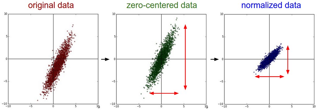Common data preprocessing pipeline. Left: Original toy, 2-dimensional input data. Middle: The data is zero-centered by subtracting the mean in each dimension. The data cloud is now centered around the origin. Right: Each dimension is additionally scaled by its standard deviation. The red lines indicate the extent of the data - they are of unequal length in the middle, but of equal length on the right.

흔한 데이터 전처리 흐름. 왼쪽: 원래의 장난감 2차원 입력 데이터. 가운데: 각 차원에서 평균을 빼 데이터를 0 중심으로 옮겼다. 이제 데이터 구름이 원점 주위에 놓인다. 오른쪽: 각 차원을 그 표준편차로 추가로 나누었다. 빨간 선은 데이터가 뻗은 범위를 나타내는데, 가운데에서는 길이가 서로 다르지만 오른쪽에서는 같다.

PCA and Whitening is another form of preprocessing. In this process, the data is first centered as described above. Then, we can compute the covariance matrix that tells us about the correlation structure in the data:

PCA와 백색화(whitening)는 또 다른 전처리 방식이다. 이 과정에서는 먼저 위에서 설명한 대로 데이터를 중심으로 옮긴다. 그런 다음 데이터 안의 상관 구조를 알려주는 공분산 행렬을 계산할 수 있다.

  
# Assume input data matrix X of size [N x D]
X -= np.mean(X, axis = 0) # zero-center the data (important)
cov = np.dot(X.T, X) / X.shape[0] # get the data covariance matrix

The (i,j) element of the data covariance matrix contains the covariance between i-th and j-th dimension of the data. In particular, the diagonal of this matrix contains the variances. Furthermore, the covariance matrix is symmetric and positive semi-definite. We can compute the SVD factorization of the data covariance matrix:

데이터 공분산 행렬의 (i,j) 원소는 데이터의 i번째 차원과 j번째 차원 사이의 공분산을 담는다. 특히 이 행렬의 대각 원소는 분산이다. 또한 공분산 행렬은 대칭이고 양의 준정부호다. 이 데이터 공분산 행렬의 SVD 분해는 다음과 같이 계산할 수 있다.

  
U,S,V = np.linalg.svd(cov)

where the columns of U are the eigenvectors and S is a 1-D array of the singular values. To decorrelate the data, we project the original (but zero-centered) data into the eigenbasis:

여기서 U의 열들은 고유벡터이고 S는 특잇값을 담은 1차원 배열이다. 데이터의 상관을 없애려면 원래의 (다만 0 중심으로 옮긴) 데이터를 고유기저로 사영한다.

  
Xrot = np.dot(X, U) # decorrelate the data

Notice that the columns of U are a set of orthonormal vectors (norm of 1, and orthogonal to each other), so they can be regarded as basis vectors. The projection therefore corresponds to a rotation of the data in X so that the new axes are the eigenvectors. If we were to compute the covariance matrix of Xrot, we would see that it is now diagonal. A nice property of np.linalg.svd is that in its returned value U, the eigenvector columns are sorted by their eigenvalues. We can use this to reduce the dimensionality of the data by only using the top few eigenvectors, and discarding the dimensions along which the data has no variance. This is also sometimes referred to as Principal Component Analysis (PCA) dimensionality reduction:

U의 열들이 정규직교 벡터의 집합(노름이 1이고 서로 직교한다)이므로 기저 벡터로 볼 수 있다는 점에 주목하자. 따라서 이 사영은 새 축이 고유벡터가 되도록 X의 데이터를 회전시키는 것에 해당한다. Xrot의 공분산 행렬을 계산해보면 이제 대각 행렬이 되어 있음을 알 수 있다. np.linalg.svd의 좋은 성질 하나는 반환값 U에서 고유벡터 열들이 고윳값 순으로 정렬되어 있다는 것이다. 이를 이용하면 상위 몇 개의 고유벡터만 쓰고 데이터의 분산이 없는 방향의 차원은 버려서 데이터의 차원을 줄일 수 있다. 이것을 주성분 분석(PCA) 차원 축소라고 부르기도 한다.

  
Xrot_reduced = np.dot(X, U[:,:100]) # Xrot_reduced becomes [N x 100]

After this operation, we would have reduced the original dataset of size [N x D] to one of size [N x 100], keeping the 100 dimensions of the data that contain the most variance. It is very often the case that you can get very good performance by training linear classifiers or neural networks on the PCA-reduced datasets, obtaining savings in both space and time.

이 연산을 거치면 원래 [N x D] 크기였던 데이터셋이 [N x 100] 크기로 줄고, 분산을 가장 많이 담은 100개 차원이 남는다. PCA로 줄인 데이터셋에 선형 분류기나 신경망을 학습시켜도 아주 좋은 성능이 나오는 경우가 매우 흔하며, 공간과 시간 양쪽에서 절약이 된다.

The last transformation you may see in practice is whitening. The whitening operation takes the data in the eigenbasis and divides every dimension by the eigenvalue to normalize the scale. The geometric interpretation of this transformation is that if the input data is a multivariable gaussian, then the whitened data will be a gaussian with zero mean and identity covariance matrix. This step would take the form:

실전에서 볼 수 있는 마지막 변환은 백색화다. 백색화 연산은 고유기저 위의 데이터를 받아 각 차원을 그 고윳값으로 나눠 크기를 정규화한다. 이 변환의 기하학적 해석은, 입력 데이터가 다변량 가우시안이라면 백색화된 데이터는 평균이 0이고 공분산 행렬이 단위 행렬인 가우시안이 된다는 것이다. 이 단계는 다음과 같은 형태가 된다.

  
# whiten the data:
# divide by the eigenvalues (which are square roots of the singular values)
Xwhite = Xrot / np.sqrt(S + 1e-5)

Warning: Exaggerating noise. Note that we’re adding 1e-5 (or a small constant) to prevent division by zero. One weakness of this transformation is that it can greatly exaggerate the noise in the data, since it stretches all dimensions (including the irrelevant dimensions of tiny variance that are mostly noise) to be of equal size in the input. This can in practice be mitigated by stronger smoothing (i.e. increasing 1e-5 to be a larger number).

경고: 잡음이 과장된다. 0으로 나누는 것을 막으려고 1e-5(또는 작은 상수)를 더하고 있다는 점에 유의하자. 이 변환의 약점 하나는 데이터의 잡음을 크게 과장할 수 있다는 것이다. 분산이 아주 작아 대부분 잡음인 무관한 차원까지 포함해 모든 차원을 입력에서 같은 크기가 되도록 늘려놓기 때문이다. 실전에서는 더 강하게 매끄럽게 만들어(즉 1e-5를 더 큰 수로 키워) 이를 완화할 수 있다.

역주. 본문은 백색화가 “각 차원을 그 고윳값으로 나눈다”고 하는데 코드는 Xrot / np.sqrt(S + 1e-5) 로 제곱근을 취하고, 코드 주석은 고윳값이 특잇값의 제곱근이라고 적어 셋이 서로 어긋나 보인다. 맞는 것은 코드다. cov 는 대칭이고 양의 준정부호인 행렬이므로 그 특잇값 S 가 곧 고윳값이며, 고유기저 위에서 Xrot 의 \(i\)번째 차원이 갖는 분산이 바로 \(S_i\)다. 분산을 1로 맞추려면 분산이 아니라 표준편차, 곧 \(\sqrt{S_i}\) 로 나눠야 한다. 이 절 첫머리에서 X /= np.std(X, axis = 0) 으로 표준편차를 나눴던 것과 똑같은 연산을 회전된 축 위에서 하는 셈이다.

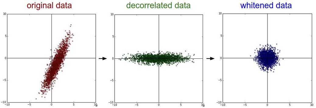PCA / Whitening. Left: Original toy, 2-dimensional input data. Middle: After performing PCA. The data is centered at zero and then rotated into the eigenbasis of the data covariance matrix. This decorrelates the data (the covariance matrix becomes diagonal). Right: Each dimension is additionally scaled by the eigenvalues, transforming the data covariance matrix into the identity matrix. Geometrically, this corresponds to stretching and squeezing the data into an isotropic gaussian blob.

PCA / 백색화. 왼쪽: 원래의 장난감 2차원 입력 데이터. 가운데: PCA를 수행한 뒤. 데이터를 0 중심으로 옮긴 다음 데이터 공분산 행렬의 고유기저로 회전시켰다. 이로써 데이터의 상관이 사라진다(공분산 행렬이 대각 행렬이 된다). 오른쪽: 각 차원을 고윳값으로 추가로 나누어 데이터 공분산 행렬을 단위 행렬로 만들었다. 기하학적으로는 데이터를 등방적인 가우시안 덩어리가 되도록 늘리고 눌러 담는 것에 해당한다.

We can also try to visualize these transformations with CIFAR-10 images. The training set of CIFAR-10 is of size 50,000 x 3072, where every image is stretched out into a 3072-dimensional row vector. We can then compute the [3072 x 3072] covariance matrix and compute its SVD decomposition (which can be relatively expensive). What do the computed eigenvectors look like visually? An image might help:

이 변환들을 CIFAR-10 이미지로 시각화해볼 수도 있다. CIFAR-10의 학습 집합은 50,000 x 3072 크기이며, 이미지 하나하나가 3072차원 행벡터로 펼쳐져 있다. 그러면 [3072 x 3072] 공분산 행렬을 계산하고 그 SVD 분해를 구할 수 있다(상당히 비쌀 수 있다). 계산된 고유벡터들은 눈으로 보면 어떤 모습일까? 그림이 도움이 될 것이다.

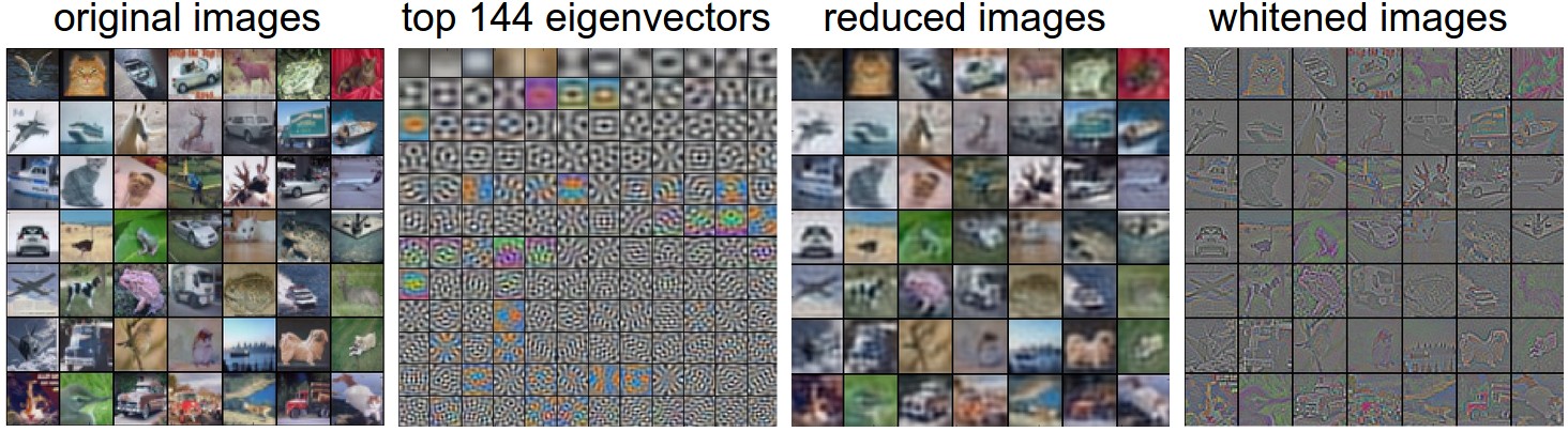Left: An example set of 49 images. 2nd from Left: The top 144 out of 3072 eigenvectors. The top eigenvectors account for most of the variance in the data, and we can see that they correspond to lower frequencies in the images. 2nd from Right: The 49 images reduced with PCA, using the 144 eigenvectors shown here. That is, instead of expressing every image as a 3072-dimensional vector where each element is the brightness of a particular pixel at some location and channel, every image above is only represented with a 144-dimensional vector, where each element measures how much of each eigenvector adds up to make up the image. In order to visualize what image information has been retained in the 144 numbers, we must rotate back into the “pixel” basis of 3072 numbers. Since U is a rotation, this can be achieved by multiplying by U.transpose()[:144,:], and then visualizing the resulting 3072 numbers as the image. You can see that the images are slightly blurrier, reflecting the fact that the top eigenvectors capture lower frequencies. However, most of the information is still preserved. Right: Visualization of the “white” representation, where the variance along every one of the 144 dimensions is squashed to equal length. Here, the whitened 144 numbers are rotated back to image pixel basis by multiplying by U.transpose()[:144,:]. The lower frequencies (which accounted for most variance) are now negligible, while the higher frequencies (which account for relatively little variance originally) become exaggerated.

왼쪽: 이미지 49개로 이루어진 예시 집합. 왼쪽에서 두 번째: 고유벡터 3072개 중 상위 144개. 상위 고유벡터가 데이터의 분산 대부분을 설명하며, 이들이 이미지의 낮은 주파수 성분에 대응한다는 것을 볼 수 있다. 오른쪽에서 두 번째: 여기 그린 고유벡터 144개를 써서 PCA로 줄인 49개 이미지. 즉 이미지 하나하나를 각 원소가 특정 위치와 채널의 픽셀 밝기인 3072차원 벡터로 나타내는 대신, 위의 이미지들은 각 원소가 그 이미지를 만드는 데 각 고유벡터가 얼마나 쓰였는지를 재는 144차원 벡터만으로 표현되어 있다. 이 144개 숫자에 어떤 이미지 정보가 남아 있는지 눈으로 보려면 3072개 숫자로 이루어진 “픽셀” 기저로 되돌려 회전시켜야 한다. U가 회전이므로 U.transpose()[:144,:]를 곱한 다음 그 결과 3072개 숫자를 이미지로 그리면 된다. 이미지가 약간 흐릿해진 것을 볼 수 있는데, 상위 고유벡터가 낮은 주파수를 담는다는 사실을 반영한다. 그래도 정보의 대부분은 여전히 보존되어 있다. 오른쪽: “백색화된” 표현의 시각화로, 144개 차원 각각의 분산을 모두 같은 길이로 눌러놓은 것이다. 여기서도 백색화된 144개 숫자에 U.transpose()[:144,:]를 곱해 이미지 픽셀 기저로 되돌렸다. (원래 분산의 대부분을 차지하던) 낮은 주파수는 이제 무시할 만해지고, (원래는 분산을 상대적으로 조금밖에 차지하지 않던) 높은 주파수는 과장된다.

In practice. We mention PCA/Whitening in these notes for completeness, but these transformations are not used with Convolutional Networks. However, it is very important to zero-center the data, and it is common to see normalization of every pixel as well.

실전에서. 이 노트에서는 완결성을 위해 PCA/백색화를 언급했지만, 이 변환들은 합성곱 신경망에서는 쓰이지 않는다. 다만 데이터를 0 중심으로 옮기는 것은 매우 중요하며, 픽셀마다 정규화하는 것도 흔히 볼 수 있다.

Common pitfall. An important point to make about the preprocessing is that any preprocessing statistics (e.g. the data mean) must only be computed on the training data, and then applied to the validation / test data. E.g. computing the mean and subtracting it from every image across the entire dataset and then splitting the data into train/val/test splits would be a mistake. Instead, the mean must be computed only over the training data and then subtracted equally from all splits (train/val/test).

흔히 빠지는 함정. 전처리에 관해 짚어둘 중요한 점은, 어떤 전처리 통계량이든(예컨대 데이터 평균) 반드시 학습 데이터에서만 계산해서 검증/테스트 데이터에 적용해야 한다는 것이다. 예컨대 데이터셋 전체에 걸쳐 평균을 구해 모든 이미지에서 뺀 다음 데이터를 학습/검증/테스트로 나누는 것은 잘못이다. 대신 평균은 학습 데이터만으로 계산한 뒤 세 갈래(학습/검증/테스트) 모두에서 똑같이 빼야 한다.

역주. 왜 잘못인지 한 줄로 말하면, 데이터셋 전체에서 구한 평균에는 검증 데이터와 테스트 데이터가 이미 섞여 들어가 있기 때문이다. 그 평균을 빼는 순간 아직 보지 말았어야 할 예제들의 정보가 학습에 쓰이는 입력을 통해 모델로 새어 들어가고, 그렇게 잰 테스트 정확도는 진짜로 처음 보는 데이터에서 나올 성능보다 낙관적으로 부풀려진다. 01번에서 “테스트 집합은 맨 마지막에 딱 한 번만 평가한다”고 했던 규칙이 전처리 단계에도 그대로 적용된다고 보면 된다. 실무에서는 학습 데이터로 계산한 평균과 표준편차를 모델 가중치와 함께 저장해 두었다가 추론할 때 그 값을 그대로 다시 쓴다. 새 데이터가 들어올 때마다 그 데이터로 평균을 다시 계산하는 것도 같은 이유로 잘못이다.

Weight Initialization

We have seen how to construct a Neural Network architecture, and how to preprocess the data. Before we can begin to train the network we have to initialize its parameters.

신경망 구조를 어떻게 짜는지, 데이터를 어떻게 전처리하는지 봤다. 신경망 학습을 시작하려면 그 전에 매개변수를 초기화해야 한다.

Pitfall: all zero initialization. Lets start with what we should not do. Note that we do not know what the final value of every weight should be in the trained network, but with proper data normalization it is reasonable to assume that approximately half of the weights will be positive and half of them will be negative. A reasonable-sounding idea then might be to set all the initial weights to zero, which we expect to be the “best guess” in expectation. This turns out to be a mistake, because if every neuron in the network computes the same output, then they will also all compute the same gradients during backpropagation and undergo the exact same parameter updates. In other words, there is no source of asymmetry between neurons if their weights are initialized to be the same.

함정: 전부 0으로 초기화하기. 하지 말아야 할 것부터 보자. 학습이 끝난 신경망에서 각 가중치의 최종 값이 얼마여야 하는지는 알 수 없지만, 데이터 정규화(normalization)를 제대로 했다면 가중치의 대략 절반은 양수이고 절반은 음수일 것이라고 가정하는 것이 합리적이다. 그렇다면 초기 가중치를 전부 0으로 두는 것이 기댓값 측면에서 “가장 나은 추측”이라는 그럴듯한 생각이 떠오를 수 있다. 그러나 이것은 잘못이다. 신경망의 모든 뉴런이 같은 출력을 계산하면 역전파 때 계산되는 기울기도 전부 같아지고 매개변수 갱신도 완전히 똑같이 일어나기 때문이다. 다시 말해 가중치를 같은 값으로 초기화하면 뉴런들 사이에 비대칭성을 만들어낼 원천이 없다.

Small random numbers. Therefore, we still want the weights to be very close to zero, but as we have argued above, not identically zero. As a solution, it is common to initialize the weights of the neurons to small numbers and refer to doing so as symmetry breaking. The idea is that the neurons are all random and unique in the beginning, so they will compute distinct updates and integrate themselves as diverse parts of the full network. The implementation for one weight matrix might look like W = 0.01* np.random.randn(D,H), where randn samples from a zero mean, unit standard deviation gaussian. With this formulation, every neuron’s weight vector is initialized as a random vector sampled from a multi-dimensional gaussian, so the neurons point in random direction in the input space. It is also possible to use small numbers drawn from a uniform distribution, but this seems to have relatively little impact on the final performance in practice.

작은 난수. 그러므로 가중치가 0에 아주 가깝기는 하되, 위에서 논한 대로 정확히 0이어서는 안 된다. 해결책으로 뉴런의 가중치를 작은 수로 초기화하는 것이 흔하며, 이를 대칭 깨기(symmetry breaking)라고 부른다. 처음에 뉴런들이 전부 무작위이고 서로 달라서 저마다 다른 갱신을 계산하며 신경망 전체의 다양한 부분으로 자리를 잡아간다는 발상이다. 가중치 행렬 하나에 대한 구현은 W = 0.01* np.random.randn(D,H) 같은 모습이 되는데, randn은 평균 0, 표준편차 1인 가우시안에서 표본을 뽑는다. 이렇게 하면 모든 뉴런의 가중치 벡터가 다차원 가우시안에서 뽑은 무작위 벡터로 초기화되므로, 뉴런들은 입력 공간에서 무작위 방향을 가리키게 된다. 균등 분포에서 뽑은 작은 수를 써도 되지만, 실전에서 최종 성능에 미치는 영향은 비교적 작아 보인다.

Warning: It’s not necessarily the case that smaller numbers will work strictly better. For example, a Neural Network layer that has very small weights will during backpropagation compute very small gradients on its data (since this gradient is proportional to the value of the weights). This could greatly diminish the “gradient signal” flowing backward through a network, and could become a concern for deep networks.

경고: 더 작은 수가 무조건 더 잘 된다는 법은 없다. 예를 들어 가중치가 아주 작은 신경망 층은 역전파 때 자기 데이터에 대해 아주 작은 기울기를 계산한다(이 기울기가 가중치 값에 비례하기 때문이다). 이는 신경망을 거슬러 흐르는 “기울기 신호”를 크게 약화시킬 수 있고, 깊은 신경망에서는 문제가 될 수 있다.

Calibrating the variances with 1/sqrt(n). One problem with the above suggestion is that the distribution of the outputs from a randomly initialized neuron has a variance that grows with the number of inputs. It turns out that we can normalize the variance of each neuron’s output to 1 by scaling its weight vector by the square root of its fan-in (i.e. its number of inputs). That is, the recommended heuristic is to initialize each neuron’s weight vector as: w = np.random.randn(n) / sqrt(n), where n is the number of its inputs. This ensures that all neurons in the network initially have approximately the same output distribution and empirically improves the rate of convergence.

1/sqrt(n)으로 분산 보정하기. 위 제안의 문제 하나는, 무작위로 초기화한 뉴런의 출력 분포가 갖는 분산이 입력 개수에 따라 커진다는 점이다. 알고 보면 각 뉴런의 가중치 벡터를 그 팬인(fan-in), 곧 입력 개수의 제곱근으로 나눠주면 출력의 분산을 1로 맞출 수 있다. 즉 권장되는 어림법은 각 뉴런의 가중치 벡터를 w = np.random.randn(n) / sqrt(n)으로 초기화하는 것이며, 여기서 n은 그 뉴런의 입력 개수다. 이렇게 하면 신경망의 모든 뉴런이 처음에 대략 같은 출력 분포를 갖게 되고, 경험적으로 수렴 속도가 개선된다.

The sketch of the derivation is as follows: Consider the inner product \(s = \sum_i^n w_i x_i\) between the weights \(w\) and input \(x\), which gives the raw activation of a neuron before the non-linearity. We can examine the variance of \(s\):
\[\begin{align} \text{Var}(s) &= \text{Var}(\sum_i^n w_ix_i) \\\\ &= \sum_i^n \text{Var}(w_ix_i) \\\\ &= \sum_i^n [E(w_i)]^2\text{Var}(x_i) + [E(x_i)]^2\text{Var}(w_i) + \text{Var}(x_i)\text{Var}(w_i) \\\\ &= \sum_i^n \text{Var}(x_i)\text{Var}(w_i) \\\\ &= \left( n \text{Var}(w) \right) \text{Var}(x) \end{align}\]

유도의 개요는 다음과 같다. 가중치 \(w\)와 입력 \(x\)의 내적 \(s = \sum_i^n w_i x_i\)를 생각하자. 이것이 비선형성을 씌우기 전 뉴런의 날것 활성값이다. \(s\)의 분산을 살펴보자.

where in the first 2 steps we have used properties of variance. In third step we assumed zero mean inputs and weights, so \(E[x_i] = E[w_i] = 0\). Note that this is not generally the case: For example ReLU units will have a positive mean. In the last step we assumed that all \(w_i, x_i\) are identically distributed. From this derivation we can see that if we want \(s\) to have the same variance as all of its inputs \(x\), then during initialization we should make sure that the variance of every weight \(w\) is \(1/n\). And since \(\text{Var}(aX) = a^2\text{Var}(X)\) for a random variable \(X\) and a scalar \(a\), this implies that we should draw from unit gaussian and then scale it by \(a = \sqrt{1/n}\), to make its variance \(1/n\). This gives the initialization w = np.random.randn(n) / sqrt(n).

처음 두 단계에서는 분산의 성질을 썼다. 세 번째 단계에서는 입력과 가중치의 평균이 0이라고 가정해 \(E[x_i] = E[w_i] = 0\)으로 두었다. 이것이 일반적으로 성립하지는 않는다는 점에 유의하자. 예컨대 ReLU 유닛은 평균이 양수다. 마지막 단계에서는 모든 \(w_i, x_i\)가 같은 분포를 따른다고 가정했다. 이 유도에서 알 수 있는 것은, \(s\)가 자기 입력 \(x\)와 같은 분산을 갖기를 바란다면 초기화할 때 모든 가중치 \(w\)의 분산이 \(1/n\)이 되도록 해야 한다는 점이다. 그리고 확률 변수 \(X\)와 스칼라 \(a\)에 대해 \(\text{Var}(aX) = a^2\text{Var}(X)\)이므로, 단위 가우시안에서 뽑은 뒤 \(a = \sqrt{1/n}\)을 곱해 분산을 \(1/n\)으로 만들어야 한다는 뜻이 된다. 여기서 w = np.random.randn(n) / sqrt(n)이라는 초기화가 나온다.

A similar analysis is carried out in Understanding the difficulty of training deep feedforward neural networks by Glorot et al. In this paper, the authors end up recommending an initialization of the form \(\text{Var}(w) = 2/(n_{in} + n_{out})\) where \(n_{in}, n_{out}\) are the number of units in the previous layer and the next layer. This is based on a compromise and an equivalent analysis of the backpropagated gradients. A more recent paper on this topic, Delving Deep into Rectifiers: Surpassing Human-Level Performance on ImageNet Classification by He et al., derives an initialization specifically for ReLU neurons, reaching the conclusion that the variance of neurons in the network should be \(2.0/n\). This gives the initialization w = np.random.randn(n) * sqrt(2.0/n), and is the current recommendation for use in practice in the specific case of neural networks with ReLU neurons.

Understanding the difficulty of training deep feedforward neural networks에서 Glorot 등이 비슷한 분석을 했다. 이 논문에서 저자들은 \(\text{Var}(w) = 2/(n_{in} + n_{out})\) 형태의 초기화를 권하는 것으로 결론짓는데, \(n_{in}, n_{out}\)은 각각 앞 층과 뒤 층의 유닛 수다. 이는 역전파된 기울기에 대해서도 같은 분석을 한 뒤 둘을 절충한 결과다. 이 주제에 관한 더 최근 논문인 He 등의 Delving Deep into Rectifiers: Surpassing Human-Level Performance on ImageNet Classification은 ReLU 뉴런에 특화된 초기화를 유도하며, 신경망에서 뉴런의 분산이 \(2.0/n\)이어야 한다는 결론에 이른다. 여기서 w = np.random.randn(n) * sqrt(2.0/n)이라는 초기화가 나오고, ReLU 뉴런을 쓰는 신경망에 한해서는 이것이 현재 실전에서 권장되는 방식이다.

역주. 계수 2가 어디서 오는지는 위 유도에 ReLU 한 줄만 얹으면 보인다. 유도는 \(\text{Var}(s) = \left( n \text{Var}(w) \right) \text{Var}(x)\)까지 왔는데, 여기서 \(x\)는 앞 층의 출력, 곧 이미 ReLU를 통과한 값이다. 0을 중심으로 대칭인 값 \(z\)에 \(\max(0, z)\)를 씌우면 절반이 0으로 잘려 나가므로
\[E[\max(0, z)^2] = \tfrac{1}{2} E[z^2]\]
가 되어 분산이 절반으로 준다. 층을 하나 지날 때마다 분산이 절반씩 깎이는 셈이니, 그 손실을 미리 메우려면 \(n \text{Var}(w)\)가 1이 아니라 2여야 하고 여기서 \(\text{Var}(w) = 2/n\)이 나온다. 절반을 잘라내지 않는 sigmoid나 tanh에는 이 계수 2가 필요 없으며, 그래서 He 초기화는 ReLU 계열에 한정된 권장 사항이다. 아래 보충에서 층을 지날 때마다 활성값이 실제로 어떻게 되는지 재본다.

Sparse initialization. Another way to address the uncalibrated variances problem is to set all weight matrices to zero, but to break symmetry every neuron is randomly connected (with weights sampled from a small gaussian as above) to a fixed number of neurons below it. A typical number of neurons to connect to may be as small as 10.

희소 초기화. 보정되지 않은 분산 문제를 다루는 또 다른 방법은 가중치 행렬을 전부 0으로 두되, 대칭을 깨기 위해 모든 뉴런을 아래쪽 뉴런 중 정해진 개수만큼과 무작위로 연결하는 것이다(연결된 가중치는 위와 같이 작은 가우시안에서 뽑는다). 연결하는 뉴런 수는 10개 정도로 적을 수도 있다.

Initializing the biases. It is possible and common to initialize the biases to be zero, since the asymmetry breaking is provided by the small random numbers in the weights. For ReLU non-linearities, some people like to use small constant value such as 0.01 for all biases because this ensures that all ReLU units fire in the beginning and therefore obtain and propagate some gradient. However, it is not clear if this provides a consistent improvement (in fact some results seem to indicate that this performs worse) and it is more common to simply use 0 bias initialization.

편향 초기화. 대칭을 깨는 일은 가중치의 작은 난수가 맡으므로 편향은 0으로 초기화해도 되고 그렇게 하는 것이 흔하다. ReLU 비선형성을 쓸 때는 모든 편향에 0.01 같은 작은 상수를 쓰기를 좋아하는 사람도 있는데, 처음에 모든 ReLU 유닛이 발화해 기울기를 얻고 전달하도록 보장하기 때문이다. 다만 이것이 꾸준한 개선을 주는지는 분명치 않으며(사실 오히려 나쁘다는 결과도 있어 보인다), 그냥 편향을 0으로 초기화하는 쪽이 더 흔하다.

In practice, the current recommendation is to use ReLU units and use the w = np.random.randn(n) * sqrt(2.0/n), as discussed in He et al..

실전에서는 ReLU 유닛을 쓰고 He 등에서 논한 대로 w = np.random.randn(n) * sqrt(2.0/n)을 쓰는 것이 현재의 권장 사항이다.

Batch Normalization. A recently developed technique by Ioffe and Szegedy called Batch Normalization alleviates a lot of headaches with properly initializing neural networks by explicitly forcing the activations throughout a network to take on a unit gaussian distribution at the beginning of the training. The core observation is that this is possible because normalization is a simple differentiable operation. In the implementation, applying this technique usually amounts to insert the BatchNorm layer immediately after fully connected layers (or convolutional layers, as we’ll soon see), and before non-linearities. We do not expand on this technique here because it is well described in the linked paper, but note that it has become a very common practice to use Batch Normalization in neural networks. In practice networks that use Batch Normalization are significantly more robust to bad initialization. Additionally, batch normalization can be interpreted as doing preprocessing at every layer of the network, but integrated into the network itself in a differentiable manner. Neat!

Batch Normalization. Ioffe와 Szegedy가 최근 개발한 Batch Normalization이라는 기법은, 학습 초기에 신경망 전체의 활성값이 단위 가우시안 분포를 따르도록 명시적으로 강제함으로써 신경망을 제대로 초기화하는 데 따르는 골칫거리를 많이 덜어준다. 핵심 관찰은 정규화(normalization)가 미분 가능한 간단한 연산이기 때문에 이것이 가능하다는 점이다. 구현에서 이 기법을 적용한다는 것은 보통 완전 연결 층(또는 곧 보게 될 합성곱 층) 바로 뒤, 비선형성 앞에 BatchNorm 층을 끼워 넣는 것을 뜻한다. 링크한 논문에 잘 설명되어 있으므로 여기서 더 펼치지는 않지만, 신경망에서 Batch Normalization을 쓰는 것이 아주 흔한 관행이 되었다는 점은 짚어둔다. 실제로 Batch Normalization을 쓴 신경망은 나쁜 초기화에 훨씬 강건하다. 또한 batch normalization은 신경망의 모든 층에서 전처리를 하되 그것을 미분 가능한 방식으로 신경망 자체에 통합한 것으로 해석할 수도 있다. 멋지다!

보충: 초기화 배율에 따라 층마다 ReLU 활성값이 어떻게 되는지 재어보기

\(1/\sqrt{n}\) 보정과 He의 \(\sqrt{2/n}\)이 실제로 무엇을 지켜주는지는 층을 여러 개 쌓아놓고 활성값의 표준편차를 층마다 재보면 한눈에 보인다. 뉴런 500개짜리 ReLU 층을 10개 쌓고, 가중치 배율만 세 가지로 바꿔가며 같은 입력을 흘려보자. 학습은 하지 않고 순전파만 한 번 한다.

  
import numpy as np

np.random.seed(0)
D, H, L = 500, 500, 10                      # 입력 500차원, 층마다 뉴런 500개, 층 10개
X = np.random.randn(1000, D)                # 예제 1000개

def activation_stds(scale):
    """초기화 배율을 바꿔가며 층을 지날 때마다 활성값의 표준편차를 잰다."""
    rng = np.random.RandomState(1)
    h, stds = X, []
    for _ in range(L):
        W = rng.randn(h.shape[1], H) * scale(h.shape[1])
        h = np.maximum(0, h.dot(W))         # ReLU
        stds.append(h.std())
    return stds

settings = [
    ("0.01 * randn      ", lambda n: 0.01),
    ("randn / sqrt(n)   ", lambda n: 1.0 / np.sqrt(n)),
    ("randn * sqrt(2/n) ", lambda n: np.sqrt(2.0 / n)),
]
print("초기화               " + "".join("%9d" % (i + 1) for i in range(L)) + "  (층)")
for name, scale in settings:
    print(name + " " + "".join("%9.4f" % s for s in activation_stds(scale)))

초기화                       1        2        3        4        5        6        7        8        9       10  (층)
0.01 * randn          0.1304   0.0207   0.0032   0.0005   0.0001   0.0000   0.0000   0.0000   0.0000   0.0000
randn / sqrt(n)       0.5834   0.4147   0.2887   0.1943   0.1284   0.0922   0.0643   0.0433   0.0299   0.0215
randn * sqrt(2/n)     0.8250   0.8293   0.8166   0.7772   0.7264   0.7373   0.7275   0.6930   0.6770   0.6884

0.01 * randn은 다섯 번째 층에서 이미 활성값이 사실상 전부 0이다. 순전파가 죽었으니 역전파로 돌아올 기울기도 없고, 원문이 “‘기울기 신호’를 크게 약화시킬 수 있다”고 경고한 상황이 그대로 재현된다. randn / sqrt(n)은 훨씬 낫지만 층마다 대략 \(1/\sqrt{2}\)배씩 줄어들어 열 번째 층에서는 처음의 4%도 남지 않는다. 위 역주에서 본 ReLU의 절반 손실이 열 번 누적된 결과다. \(\sqrt{2.0/n}\)을 쓰면 그 절반이 계수 2로 정확히 상쇄되어 열 층을 지나도 표준편차가 0.7 언저리에 머문다. 초기화 배율 하나만 바꿨을 뿐인데 신경망이 신호를 통과시키느냐 아니냐가 갈린다. 바로 앞 문단의 Batch Normalization은 이 표를 초기화 배율로 맞추는 대신 층 안에서 매번 강제로 맞춰버리는 방법이라고 보면 된다. 원문이 “나쁜 초기화에 훨씬 강건하다”고 말한 것이 이 뜻이다.

Regularization

There are several ways of controlling the capacity of Neural Networks to prevent overfitting:

신경망이 과적합하지 않도록 그 수용력을 다스리는 방법에는 여러 가지가 있다.

L2 regularization is perhaps the most common form of regularization. It can be implemented by penalizing the squared magnitude of all parameters directly in the objective. That is, for every weight \(w\) in the network, we add the term \(\frac{1}{2} \lambda w^2\) to the objective, where \(\lambda\) is the regularization strength. It is common to see the factor of \(\frac{1}{2}\) in front because then the gradient of this term with respect to the parameter \(w\) is simply \(\lambda w\) instead of \(2 \lambda w\). The L2 regularization has the intuitive interpretation of heavily penalizing peaky weight vectors and preferring diffuse weight vectors. As we discussed in the Linear Classification section, due to multiplicative interactions between weights and inputs this has the appealing property of encouraging the network to use all of its inputs a little rather than some of its inputs a lot. Lastly, notice that during gradient descent parameter update, using the L2 regularization ultimately means that every weight is decayed linearly: W += -lambda * W towards zero.

L2 정규화(regularization)는 아마도 가장 흔한 형태의 정규화일 것이다. 모든 매개변수의 제곱 크기에 목적 함수에서 곧바로 벌점을 매겨 구현할 수 있다. 즉 신경망의 모든 가중치 \(w\)에 대해 \(\frac{1}{2} \lambda w^2\) 항을 목적 함수에 더하며, \(\lambda\)는 정규화 세기다. 앞에 \(\frac{1}{2}\)이 붙은 것을 흔히 보게 되는데, 그러면 이 항을 매개변수 \(w\)로 미분한 기울기가 \(2 \lambda w\)가 아니라 그냥 \(\lambda w\)가 되기 때문이다. L2 정규화는 뾰족한 가중치 벡터에 무거운 벌점을 매기고 널리 퍼진 가중치 벡터를 선호한다는 직관적 해석을 갖는다. 선형 분류 절에서 이야기했듯, 가중치와 입력이 곱셈으로 상호작용하는 덕분에 이는 신경망이 일부 입력만 많이 쓰기보다 모든 입력을 조금씩 쓰도록 유도한다는 매력적인 성질을 갖는다. 마지막으로, 경사 하강법으로 매개변수를 갱신할 때 L2 정규화를 쓰면 결국 모든 가중치가 W += -lambda * W로 0을 향해 선형적으로 감쇠한다는 점에 주목하자.

L1 regularization is another relatively common form of regularization, where for each weight \(w\) we add the term \(\lambda \mid w \mid\) to the objective. It is possible to combine the L1 regularization with the L2 regularization: \(\lambda_1 \mid w \mid + \lambda_2 w^2\) (this is called Elastic net regularization). The L1 regularization has the intriguing property that it leads the weight vectors to become sparse during optimization (i.e. very close to exactly zero). In other words, neurons with L1 regularization end up using only a sparse subset of their most important inputs and become nearly invariant to the “noisy” inputs. In comparison, final weight vectors from L2 regularization are usually diffuse, small numbers. In practice, if you are not concerned with explicit feature selection, L2 regularization can be expected to give superior performance over L1.

L1 정규화는 또 하나의 비교적 흔한 형태의 정규화로, 각 가중치 \(w\)에 대해 \(\lambda \mid w \mid\) 항을 목적 함수에 더한다. L1 정규화를 L2 정규화와 결합할 수도 있다. \(\lambda_1 \mid w \mid + \lambda_2 w^2\)가 그것이며 Elastic net 정규화라고 부른다. L1 정규화에는 최적화 도중 가중치 벡터가 희소해진다(즉 정확히 0에 매우 가까워진다)는 흥미로운 성질이 있다. 다시 말해 L1 정규화를 쓴 뉴런은 자기 입력 중 가장 중요한 희소한 부분집합만 쓰게 되고 “잡음” 섞인 입력에는 거의 불변이 된다. 이에 비해 L2 정규화에서 나온 최종 가중치 벡터는 보통 작은 값들이 널리 퍼져 있는 모습이다. 실전에서 명시적인 특징 선택이 목적이 아니라면 L2 정규화가 L1보다 나은 성능을 낼 것이라고 기대할 수 있다.

역주. L1은 가중치를 정확히 0으로 만드는데 L2는 그러지 못하는 이유는 두 벌점의 기울기 모양에 있다. L2 항 \(\frac{1}{2}\lambda w^2\)의 기울기는 \(\lambda w\)라서 \(w\)가 0에 가까워질수록 함께 사그라들고, 그래서 아주 작지만 0은 아닌 값에서 멈춘다. 반면 L1 항 \(\lambda \mid w \mid\)의 기울기는 \(w\)의 크기와 무관하게 언제나 \(\pm\lambda\)여서 0 바로 옆에서도 같은 힘으로 0을 향해 민다. 데이터 손실이 그 가중치를 \(\lambda\)보다 약한 힘으로 붙잡고 있으면 결국 0에 눌러앉아 다시 나오지 못한다. 원문이 L1을 ‘명시적인 특징 선택’과 묶어 말하는 이유가 이것이다.

Max norm constraints. Another form of regularization is to enforce an absolute upper bound on the magnitude of the weight vector for every neuron and use projected gradient descent to enforce the constraint. In practice, this corresponds to performing the parameter update as normal, and then enforcing the constraint by clamping the weight vector \(\vec{w}\) of every neuron to satisfy \(\Vert \vec{w} \Vert_2 < c\). Typical values of \(c\) are on orders of 3 or 4. Some people report improvements when using this form of regularization. One of its appealing properties is that network cannot “explode” even when the learning rates are set too high because the updates are always bounded.

Max norm 제약. 또 다른 정규화 형태는 모든 뉴런의 가중치 벡터 크기에 절대적인 상한을 두고 사영 경사 하강법으로 그 제약을 지키게 하는 것이다. 실제로는 매개변수 갱신을 평소대로 한 다음, 모든 뉴런의 가중치 벡터 \(\vec{w}\)가 \(\Vert \vec{w} \Vert_2 < c\)를 만족하도록 잘라내어 제약을 강제한다. \(c\)의 전형적인 값은 3이나 4 정도다. 이 형태의 정규화로 개선을 봤다는 보고가 있다. 매력적인 성질 하나는 갱신량이 언제나 유계이므로 학습률을 너무 크게 잡아도 신경망이 “폭발”할 수 없다는 점이다.

Dropout is an extremely effective, simple and recently introduced regularization technique by Srivastava et al. in Dropout: A Simple Way to Prevent Neural Networks from Overfitting (pdf) that complements the other methods (L1, L2, maxnorm). While training, dropout is implemented by only keeping a neuron active with some probability \(p\) (a hyperparameter), or setting it to zero otherwise.

Dropout은 Srivastava 등이 Dropout: A Simple Way to Prevent Neural Networks from Overfitting(pdf)에서 최근 소개한, 대단히 효과적이고 간단한 정규화 기법으로 다른 방법들(L1, L2, maxnorm)을 보완한다. 학습 중에 dropout은 각 뉴런을 확률 \(p\)(하이퍼파라미터다)로만 활성 상태로 남기고 그렇지 않으면 0으로 두는 방식으로 구현된다.

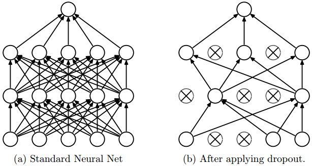Figure taken from the Dropout paper that illustrates the idea. During training, Dropout can be interpreted as sampling a Neural Network within the full Neural Network, and only updating the parameters of the sampled network based on the input data. (However, the exponential number of possible sampled networks are not independent because they share the parameters.) During testing there is no dropout applied, with the interpretation of evaluating an averaged prediction across the exponentially-sized ensemble of all sub-networks (more about ensembles in the next section).

착상을 보여주는 Dropout 논문의 그림. 학습 중 Dropout은 전체 신경망 안에서 신경망 하나를 표본으로 뽑아, 입력 데이터를 바탕으로 그 표본 신경망의 매개변수만 갱신하는 것으로 해석할 수 있다. (다만 표본으로 뽑힐 수 있는 지수적으로 많은 신경망들은 매개변수를 공유하므로 서로 독립이 아니다.) 테스트 때는 dropout을 적용하지 않는데, 지수적으로 많은 모든 부분 신경망으로 이루어진 앙상블의 예측을 평균 낸 것을 평가한다는 해석이 붙는다(앙상블은 다음 절에서 더 다룬다).

Vanilla dropout in an example 3-layer Neural Network would be implemented as follows:

예제 3층 신경망에서 바닐라 dropout은 다음과 같이 구현될 것이다.

  
""" Vanilla Dropout: Not recommended implementation (see notes below) """

p = 0.5 # probability of keeping a unit active. higher = less dropout

def train_step(X):
  """ X contains the data """
  
  # forward pass for example 3-layer neural network
  H1 = np.maximum(0, np.dot(W1, X) + b1)
  U1 = np.random.rand(*H1.shape) < p # first dropout mask
  H1 *= U1 # drop!
  H2 = np.maximum(0, np.dot(W2, H1) + b2)
  U2 = np.random.rand(*H2.shape) < p # second dropout mask
  H2 *= U2 # drop!
  out = np.dot(W3, H2) + b3
  
  # backward pass: compute gradients... (not shown)
  # perform parameter update... (not shown)
  
def predict(X):
  # ensembled forward pass
  H1 = np.maximum(0, np.dot(W1, X) + b1) * p # NOTE: scale the activations
  H2 = np.maximum(0, np.dot(W2, H1) + b2) * p # NOTE: scale the activations
  out = np.dot(W3, H2) + b3

In the code above, inside the train_step function we have performed dropout twice: on the first hidden layer and on the second hidden layer. It is also possible to perform dropout right on the input layer, in which case we would also create a binary mask for the input X. The backward pass remains unchanged, but of course has to take into account the generated masks U1,U2.

위 코드의 train_step 함수 안에서는 dropout을 두 번, 첫 번째 은닉층과 두 번째 은닉층에 수행했다. 입력층에 바로 dropout을 걸 수도 있는데, 그러면 입력 X에 대해서도 이진 마스크를 만들게 된다. 역전파는 그대로지만 물론 생성된 마스크 U1,U2를 고려해야 한다.

Crucially, note that in the predict function we are not dropping anymore, but we are performing a scaling of both hidden layer outputs by \(p\). This is important because at test time all neurons see all their inputs, so we want the outputs of neurons at test time to be identical to their expected outputs at training time. For example, in case of \(p = 0.5\), the neurons must halve their outputs at test time to have the same output as they had during training time (in expectation). To see this, consider an output of a neuron \(x\) (before dropout). With dropout, the expected output from this neuron will become \(px + (1-p)0\), because the neuron’s output will be set to zero with probability \(1-p\). At test time, when we keep the neuron always active, we must adjust \(x \rightarrow px\) to keep the same expected output. It can also be shown that performing this attenuation at test time can be related to the process of iterating over all the possible binary masks (and therefore all the exponentially many sub-networks) and computing their ensemble prediction.

결정적으로, predict 함수에서는 더 이상 뉴런을 떨어뜨리지 않는 대신 두 은닉층의 출력에 \(p\)를 곱해 크기를 조정하고 있다는 점에 주목하자. 이것이 중요한 이유는 테스트 때는 모든 뉴런이 자기 입력을 전부 보게 되므로, 테스트 때 뉴런의 출력이 학습 때의 기대 출력과 같아지기를 바라기 때문이다. 예컨대 \(p = 0.5\)라면 뉴런은 테스트 때 출력을 절반으로 줄여야 (기댓값 기준으로) 학습 때와 같은 출력을 갖는다. 이를 확인하려면 (dropout 이전의) 뉴런 출력 \(x\)를 생각해보자. dropout이 있으면 이 뉴런의 기대 출력은 \(px + (1-p)0\)이 되는데, 뉴런의 출력이 확률 \(1-p\)로 0이 되기 때문이다. 테스트 때 뉴런을 항상 활성 상태로 둔다면 같은 기대 출력을 유지하기 위해 \(x \rightarrow px\)로 조정해야 한다. 테스트 때 이렇게 값을 줄이는 것이, 가능한 모든 이진 마스크를(따라서 지수적으로 많은 모든 부분 신경망을) 훑으며 그 앙상블 예측을 계산하는 과정과 관련지어질 수 있다는 것도 보일 수 있다.

The undesirable property of the scheme presented above is that we must scale the activations by \(p\) at test time. Since test-time performance is so critical, it is always preferable to use inverted dropout, which performs the scaling at train time, leaving the forward pass at test time untouched. Additionally, this has the appealing property that the prediction code can remain untouched when you decide to tweak where you apply dropout, or if at all. Inverted dropout looks as follows:

위에서 제시한 방식의 달갑지 않은 성질은 테스트 때 활성값에 \(p\)를 곱해야 한다는 것이다. 테스트 시점의 성능은 매우 중요하므로, 크기 조정을 학습 때 수행하고 테스트 때의 순전파는 건드리지 않는 inverted dropout을 쓰는 편이 언제나 낫다. 게다가 이렇게 하면 dropout을 어디에 적용할지, 아니면 아예 적용하지 않을지를 바꿔도 예측 코드는 그대로 둘 수 있다는 매력적인 성질도 생긴다. inverted dropout은 다음과 같은 모습이다.

  
""" 
Inverted Dropout: Recommended implementation example.
We drop and scale at train time and don't do anything at test time.
"""

p = 0.5 # probability of keeping a unit active. higher = less dropout

def train_step(X):
  # forward pass for example 3-layer neural network
  H1 = np.maximum(0, np.dot(W1, X) + b1)
  U1 = (np.random.rand(*H1.shape) < p) / p # first dropout mask. Notice /p!
  H1 *= U1 # drop!
  H2 = np.maximum(0, np.dot(W2, H1) + b2)
  U2 = (np.random.rand(*H2.shape) < p) / p # second dropout mask. Notice /p!
  H2 *= U2 # drop!
  out = np.dot(W3, H2) + b3
  
  # backward pass: compute gradients... (not shown)
  # perform parameter update... (not shown)
  
def predict(X):
  # ensembled forward pass
  H1 = np.maximum(0, np.dot(W1, X) + b1) # no scaling necessary
  H2 = np.maximum(0, np.dot(W2, H1) + b2)
  out = np.dot(W3, H2) + b3

There has a been a large amount of research after the first introduction of dropout that tries to understand the source of its power in practice, and its relation to the other regularization techniques. Recommended further reading for an interested reader includes:

dropout이 처음 소개된 뒤로 그 위력이 실전에서 어디에서 오는지, 그리고 다른 정규화 기법들과 어떤 관계인지를 이해하려는 연구가 많이 이루어졌다. 관심 있는 독자에게 권하는 읽을거리는 다음과 같다.

Dropout paper by Srivastava et al. 2014.
Dropout Training as Adaptive Regularization: “we show that the dropout regularizer is first-order equivalent to an L2 regularizer applied after scaling the features by an estimate of the inverse diagonal Fisher information matrix”.

Srivastava 등이 2014년에 쓴 Dropout 논문.
Dropout Training as Adaptive Regularization: “우리는 dropout 정규화 항이, 역대각 피셔 정보 행렬의 추정값으로 특징의 크기를 조정한 뒤 적용한 L2 정규화 항과 1차 근사에서 동등함을 보인다”.

Theme of noise in forward pass. Dropout falls into a more general category of methods that introduce stochastic behavior in the forward pass of the network. During testing, the noise is marginalized over analytically (as is the case with dropout when multiplying by \(p\)), or numerically (e.g. via sampling, by performing several forward passes with different random decisions and then averaging over them). An example of other research in this direction includes DropConnect, where a random set of weights is instead set to zero during forward pass. As foreshadowing, Convolutional Neural Networks also take advantage of this theme with methods such as stochastic pooling, fractional pooling, and data augmentation. We will go into details of these methods later.

순전파에 잡음을 넣는다는 주제. dropout은 신경망의 순전파에 확률적 동작을 도입하는 더 일반적인 방법 부류에 속한다. 테스트 때는 이 잡음을 해석적으로(dropout에서 \(p\)를 곱하는 것이 그렇다) 또는 수치적으로(예컨대 표본을 뽑아, 무작위 결정을 달리한 순전파를 여러 번 수행한 뒤 평균 내어) 주변화해 없앤다. 이 방향의 다른 연구로는 DropConnect가 있는데, 순전파 때 무작위로 고른 가중치 집합을 대신 0으로 둔다. 앞질러 말하자면 합성곱 신경망도 stochastic pooling, fractional pooling, 데이터 증강 같은 방법으로 이 주제를 활용한다. 이 방법들은 뒤에서 자세히 다룬다.

Bias regularization. As we already mentioned in the Linear Classification section, it is not common to regularize the bias parameters because they do not interact with the data through multiplicative interactions, and therefore do not have the interpretation of controlling the influence of a data dimension on the final objective. However, in practical applications (and with proper data preprocessing) regularizing the bias rarely leads to significantly worse performance. This is likely because there are very few bias terms compared to all the weights, so the classifier can “afford to” use the biases if it needs them to obtain a better data loss.

편향 정규화. 선형 분류 절에서 이미 언급했듯, 편향 매개변수는 데이터와 곱셈으로 상호작용하지 않으므로 어떤 데이터 차원이 최종 목적 함수에 미치는 영향을 조절한다는 해석을 갖지 않고, 그래서 편향을 정규화하는 것은 흔하지 않다. 다만 실제 응용에서는 (그리고 데이터 전처리를 제대로 했다면) 편향을 정규화해도 성능이 크게 나빠지는 일은 드물다. 전체 가중치에 비해 편향 항이 아주 적어서, 더 나은 데이터 손실을 얻는 데 편향이 필요하다면 분류기가 그것을 “쓸 여유가 있기” 때문일 것이다.

Per-layer regularization. It is not very common to regularize different layers to different amounts (except perhaps the output layer). Relatively few results regarding this idea have been published in the literature.

층별 정규화. 층마다 정규화 양을 다르게 주는 것은 (출력층은 예외일 수 있지만) 그리 흔하지 않다. 이 착상에 관해 발표된 결과도 비교적 적다.

In practice: It is most common to use a single, global L2 regularization strength that is cross-validated. It is also common to combine this with dropout applied after all layers. The value of \(p = 0.5\) is a reasonable default, but this can be tuned on validation data.

실전에서는 교차 검증으로 정한 전역 L2 정규화 세기 하나를 쓰는 것이 가장 흔하다. 여기에 모든 층 뒤에 dropout을 적용해 함께 쓰는 것도 흔하다. \(p = 0.5\)가 합리적인 기본값이지만 검증 데이터로 조정할 수 있다.

보충: inverted dropout이 학습과 테스트에서 기댓값을 지키는지 재어보기

dropout에서 실수가 나오는 자리는 거의 언제나 학습과 테스트의 비대칭을 맞추는 부분이다. 어떤 층의 활성값을 놓고 dropout을 세 번 통과시켜, 두 구현이 각각 어떤 평균을 내는지 직접 재보자.

  
import numpy as np

np.random.seed(0)
p, N, H, L = 0.5, 2000, 400, 3              # 유지 확률 0.5, dropout 을 건 층 3개
X = np.abs(np.random.randn(N, H))           # 어떤 층에 들어오는 ReLU 활성값

def run(train_mask):
    a = X
    for _ in range(L):
        a = a * train_mask(a.shape)
    return a.mean()

vanilla  = run(lambda s: (np.random.rand(*s) < p))        # 마스크만 씌운다
inverted = run(lambda s: (np.random.rand(*s) < p) / p)    # 마스크를 p 로 나눈다

print("dropout 을 걸지 않은 활성값 평균          : %.4f" % X.mean())
print()
print("바닐라  · 학습 때 3개 층 통과 후 평균     : %.4f" % vanilla)
print("바닐라  · 테스트 때 층마다 p 를 곱하면    : %.4f" % (X.mean() * p ** L))
print("바닐라  · 테스트 때 p 곱하기를 잊으면     : %.4f  (%.1f배)"
      % (X.mean(), X.mean() / vanilla))
print()
print("inverted · 학습 때 3개 층 통과 후 평균    : %.4f" % inverted)
print("inverted · 테스트 때 아무것도 하지 않으면 : %.4f" % X.mean())

dropout 을 걸지 않은 활성값 평균          : 0.7974

바닐라  · 학습 때 3개 층 통과 후 평균     : 0.1006
바닐라  · 테스트 때 층마다 p 를 곱하면    : 0.0997
바닐라  · 테스트 때 p 곱하기를 잊으면     : 0.7974  (7.9배)

inverted · 학습 때 3개 층 통과 후 평균    : 0.7943
inverted · 테스트 때 아무것도 하지 않으면 : 0.7974

바닐라 구현은 테스트 때 층마다 \(p\)를 곱해줘야만 학습 때의 0.1006과 맞아떨어진다. 그 곱하기를 한 층에서 빠뜨리면 그만큼 활성값이 \(1/p\)인 2배로 부풀고, 세 층 모두에서 빠뜨리면 \(1/p^3\)인 8배까지 부푸는 식으로, 층이 깊어질수록 그 배수가 지수적으로 커진다. 가중치는 그대로인데 예측만 무너지는 셈이라 원인을 찾기도 어렵다. inverted dropout은 그 나눗셈을 학습 쪽으로 옮겨놓았기 때문에 학습 때 평균이 이미 dropout 없는 값과 같고, 테스트 코드는 dropout을 아예 모르는 채로 두어도 된다. 요즘 프레임워크에서 model.eval()이나 training=False가 하는 일이 바로 학습 때만 걸던 이 마스크를 꺼주는 것이며, 그것을 잊었을 때 나타나는 증상이 위 표의 어긋난 숫자들이다.

Loss functions

We have discussed the regularization loss part of the objective, which can be seen as penalizing some measure of complexity of the model. The second part of an objective is the data loss, which in a supervised learning problem measures the compatibility between a prediction (e.g. the class scores in classification) and the ground truth label. The data loss takes the form of an average over the data losses for every individual example. That is, \(L = \frac{1}{N} \sum_i L_i\) where \(N\) is the number of training data. Lets abbreviate \(f = f(x_i; W)\) to be the activations of the output layer in a Neural Network. There are several types of problems you might want to solve in practice:

목적 함수 중 정규화 손실 부분을 다뤘는데, 이는 모델의 복잡도를 재는 어떤 척도에 벌점을 매기는 것으로 볼 수 있다. 목적 함수의 두 번째 부분은 데이터 손실로, 지도 학습 문제에서 예측(예컨대 분류에서의 클래스 점수)과 ground truth 레이블이 얼마나 맞아떨어지는지를 잰다. 데이터 손실은 예제 하나하나의 데이터 손실을 평균 낸 형태다. 즉 \(L = \frac{1}{N} \sum_i L_i\)이며 \(N\)은 학습 데이터의 개수다. 신경망 출력층의 활성값을 \(f = f(x_i; W)\)로 줄여 쓰자. 실전에서 풀고 싶어질 만한 문제에는 여러 종류가 있다.

Classification is the case that we have so far discussed at length. Here, we assume a dataset of examples and a single correct label (out of a fixed set) for each example. One of two most commonly seen cost functions in this setting is the SVM (e.g. the Weston Watkins formulation):
\[L_i = \sum_{j\neq y_i} \max(0, f_j - f_{y_i} + 1)\]

분류는 지금까지 길게 다뤄온 경우다. 여기서는 예제들의 데이터셋이 있고 각 예제마다 (정해진 집합에서 나온) 정답 레이블이 하나씩 있다고 가정한다. 이 상황에서 가장 흔히 보는 비용 함수 두 가지 중 하나는 SVM이다(예컨대 Weston Watkins 형태).

As we briefly alluded to, some people report better performance with the squared hinge loss (i.e. instead using \(\max(0, f_j - f_{y_i} + 1)^2\)). The second common choice is the Softmax classifier that uses the cross-entropy loss:
\[L_i = -\log\left(\frac{e^{f_{y_i}}}{ \sum_j e^{f_j} }\right)\]

앞서 짧게 언급했듯 squared hinge loss(즉 \(\max(0, f_j - f_{y_i} + 1)^2\)를 대신 쓰는 것)로 더 나은 성능을 봤다는 보고도 있다. 두 번째로 흔한 선택지는 교차 엔트로피 손실을 쓰는 Softmax 분류기다.

Problem: Large number of classes. When the set of labels is very large (e.g. words in English dictionary, or ImageNet which contains 22,000 categories), computing the full softmax probabilities becomes expensive. For certain applications, approximate versions are popular. For instance, it may be helpful to use Hierarchical Softmax in natural language processing tasks (see one explanation here (pdf)). The hierarchical softmax decomposes words as labels in a tree. Each label is then represented as a path along the tree, and a Softmax classifier is trained at every node of the tree to disambiguate between the left and right branch. The structure of the tree strongly impacts the performance and is generally problem-dependent.

문제: 클래스가 아주 많을 때. 레이블 집합이 매우 클 때(예컨대 영어 사전의 단어들이나 22,000개 카테고리를 담은 ImageNet) 전체 softmax 확률을 계산하는 것은 비싸진다. 어떤 응용에서는 근사 버전이 널리 쓰인다. 예를 들어 자연어 처리 과제에서는 Hierarchical Softmax를 쓰는 것이 도움이 될 수 있다(여기(pdf)에 설명이 하나 있다). hierarchical softmax는 레이블인 단어들을 트리로 분해한다. 그러면 각 레이블은 트리를 따라가는 경로로 표현되고, 트리의 모든 노드마다 왼쪽 가지와 오른쪽 가지를 가려내는 Softmax 분류기를 학습시킨다. 트리의 구조가 성능에 큰 영향을 주며 대체로 문제에 따라 달라진다.

Attribute classification. Both losses above assume that there is a single correct answer \(y_i\). But what if \(y_i\) is a binary vector where every example may or may not have a certain attribute, and where the attributes are not exclusive? For example, images on Instagram can be thought of as labeled with a certain subset of hashtags from a large set of all hashtags, and an image may contain multiple. A sensible approach in this case is to build a binary classifier for every single attribute independently. For example, a binary classifier for each category independently would take the form:
\[L_i = \sum_j \max(0, 1 - y_{ij} f_j)\]

속성 분류. 위의 두 손실은 모두 정답 \(y_i\)가 하나뿐이라고 가정한다. 그런데 \(y_i\)가 이진 벡터여서, 각 예제가 어떤 속성을 가질 수도 있고 갖지 않을 수도 있으며 그 속성들이 서로 배타적이지도 않다면 어떨까? 예를 들어 인스타그램의 이미지는 전체 해시태그 집합에서 뽑은 어떤 부분집합으로 레이블이 붙어 있다고 볼 수 있고, 한 이미지에 여러 개가 달릴 수 있다. 이럴 때 합리적인 접근은 속성 하나하나마다 독립적인 이진 분류기를 만드는 것이다. 예컨대 각 카테고리마다 독립적인 이진 분류기는 다음과 같은 형태가 된다.

where the sum is over all categories \(j\), and \(y_{ij}\) is either +1 or -1 depending on whether the i-th example is labeled with the j-th attribute, and the score vector \(f_j\) will be positive when the class is predicted to be present and negative otherwise. Notice that loss is accumulated if a positive example has score less than +1, or when a negative example has score greater than -1.

여기서 합은 모든 카테고리 \(j\)에 대한 것이고, \(y_{ij}\)는 i번째 예제에 j번째 속성이 붙어 있는지에 따라 +1 또는 -1이다. 점수 벡터 \(f_j\)는 그 클래스가 있다고 예측되면 양수, 아니면 음수가 된다. 양성 예제의 점수가 +1보다 작거나 음성 예제의 점수가 -1보다 크면 손실이 쌓인다는 점에 주목하자.

An alternative to this loss would be to train a logistic regression classifier for every attribute independently. A binary logistic regression classifier has only two classes (0,1), and calculates the probability of class 1 as:
\[P(y = 1 \mid x; w, b) = \frac{1}{1 + e^{-(w^Tx +b)}} = \sigma (w^Tx + b)\]

이 손실의 대안은 속성마다 독립적으로 로지스틱 회귀 분류기를 학습시키는 것이다. 이진 로지스틱 회귀 분류기는 클래스가 (0,1) 둘뿐이며 클래스 1일 확률을 다음과 같이 계산한다.

Since the probabilities of class 1 and 0 sum to one, the probability for class 0 is \(P(y = 0 \mid x; w, b) = 1 - P(y = 1 \mid x; w,b)\). Hence, an example is classified as a positive example (y = 1) if \(\sigma (w^Tx + b) > 0.5\), or equivalently if the score \(w^Tx +b > 0\). The loss function then maximizes this probability. You can convince yourself that this simplifies to minimizing the negative log-likelihood:
\[L_i = -\sum_j y_{ij} \log(\sigma(f_j)) + (1 - y_{ij}) \log(1 - \sigma(f_j))\]

클래스 1과 클래스 0의 확률을 더하면 1이므로 클래스 0의 확률은 \(P(y = 0 \mid x; w, b) = 1 - P(y = 1 \mid x; w,b)\)이다. 따라서 \(\sigma (w^Tx + b) > 0.5\)이면, 다시 말해 점수 \(w^Tx +b > 0\)이면 그 예제는 양성 예제(y = 1)로 분류된다. 그러면 손실 함수는 이 확률을 최대화한다. 조금 정리해보면 이것이 음의 로그 가능도를 최소화하는 것으로 간단해진다는 것을 스스로 납득할 수 있다.

where the labels \(y_{ij}\) are assumed to be either 1 (positive) or 0 (negative), and \(\sigma(\cdot)\) is the sigmoid function. The expression above can look scary but the gradient on \(f\) is in fact extremely simple and intuitive: \(\partial{L_i} / \partial{f_j} = \sigma(f_j) - y_{ij}\) (as you can double check yourself by taking the derivatives).

여기서 레이블 \(y_{ij}\)는 1(양성) 또는 0(음성)이라고 가정하며 \(\sigma(\cdot)\)는 sigmoid 함수다. 위 식은 무섭게 보일 수 있지만 \(f\)에 대한 기울기는 사실 극히 간단하고 직관적이다. \(\partial{L_i} / \partial{f_j} = \sigma(f_j) - y_{ij}\)이며, 직접 미분해보면 확인할 수 있다.

Regression is the task of predicting real-valued quantities, such as the price of houses or the length of something in an image. For this task, it is common to compute the loss between the predicted quantity and the true answer and then measure the L2 squared norm, or L1 norm of the difference. The L2 norm squared would compute the loss for a single example of the form:
\[L_i = \Vert f - y_i \Vert_2^2\]

회귀는 집값이나 이미지 속 무언가의 길이처럼 실숫값을 예측하는 과제다. 이 과제에서는 예측한 양과 실제 답 사이의 손실을 구한 다음 그 차이의 L2 노름 제곱이나 L1 노름을 재는 것이 흔하다. L2 노름의 제곱을 쓰면 예제 하나에 대한 손실이 다음과 같은 형태가 된다.

The reason the L2 norm is squared in the objective is that the gradient becomes much simpler, without changing the optimal parameters since squaring is a monotonic operation. The L1 norm would be formulated by summing the absolute value along each dimension:
\[L_i = \Vert f - y_i \Vert_1 = \sum_j \mid f_j - (y_i)_j \mid\]

목적 함수에서 L2 노름을 제곱하는 이유는 기울기가 훨씬 간단해지기 때문이며, 제곱은 단조 연산이라 최적 매개변수는 달라지지 않는다. L1 노름은 각 차원의 절댓값을 더해 만든다.

where the sum \(\sum_j\) is a sum over all dimensions of the desired prediction, if there is more than one quantity being predicted. Looking at only the j-th dimension of the i-th example and denoting the difference between the true and the predicted value by \(\delta_{ij}\), the gradient for this dimension (i.e. \(\partial{L_i} / \partial{f_j}\)) is easily derived to be either \(\delta_{ij}\) with the L2 norm, or \(sign(\delta_{ij})\). That is, the gradient on the score will either be directly proportional to the difference in the error, or it will be fixed and only inherit the sign of the difference.

여기서 합 \(\sum_j\)는 예측하려는 양이 둘 이상일 때 그 예측의 모든 차원에 대한 합이다. i번째 예제의 j번째 차원만 보고 실제 값과 예측 값의 차이를 \(\delta_{ij}\)로 쓰면, 이 차원에 대한 기울기(즉 \(\partial{L_i} / \partial{f_j}\))는 L2 노름에서는 \(\delta_{ij}\), L1 노름에서는 \(sign(\delta_{ij})\)로 쉽게 유도된다. 즉 점수에 대한 기울기는 오차의 차이에 곧바로 비례하거나, 아니면 크기가 고정된 채 차이의 부호만 물려받는다.

Word of caution: It is important to note that the L2 loss is much harder to optimize than a more stable loss such as Softmax. Intuitively, it requires a very fragile and specific property from the network to output exactly one correct value for each input (and its augmentations). Notice that this is not the case with Softmax, where the precise value of each score is less important: It only matters that their magnitudes are appropriate. Additionally, the L2 loss is less robust because outliers can introduce huge gradients. When faced with a regression problem, first consider if it is absolutely inadequate to quantize the output into bins. For example, if you are predicting star rating for a product, it might work much better to use 5 independent classifiers for ratings of 1-5 stars instead of a regression loss. Classification has the additional benefit that it can give you a distribution over the regression outputs, not just a single output with no indication of its confidence. If you’re certain that classification is not appropriate, use the L2 but be careful: For example, the L2 is more fragile and applying dropout in the network (especially in the layer right before the L2 loss) is not a great idea.

한마디 주의: L2 손실이 Softmax처럼 더 안정적인 손실보다 최적화하기 훨씬 어렵다는 점은 짚어둘 필요가 있다. 직관적으로 L2 손실은 입력(과 그 증강본) 하나하나마다 정확히 하나의 옳은 값을 내놓아야 한다는, 아주 깨지기 쉽고 까다로운 성질을 신경망에 요구한다. Softmax에서는 그렇지 않다는 점에 주목하자. 거기서는 각 점수의 정확한 값이 덜 중요하고 그 크기 관계만 적절하면 된다. 게다가 L2 손실은 이상치가 거대한 기울기를 만들어낼 수 있어 덜 강건하다. 회귀 문제를 마주하면 출력을 구간으로 이산화하는 것이 정말로 부적절한지부터 먼저 생각해보라. 예컨대 어떤 상품의 별점을 예측한다면, 회귀 손실 대신 1점부터 5점까지 별점마다 독립적인 분류기 5개를 쓰는 편이 훨씬 잘 될 수도 있다. 분류에는 회귀 출력에 대한 분포를 얻을 수 있다는 이점도 있다. 확신도에 대한 아무 단서 없이 출력 하나만 나오는 것과 다르다. 분류가 적절하지 않다고 확신한다면 L2를 쓰되 조심하라. 예를 들어 L2는 더 깨지기 쉬우므로 신경망에 dropout을 적용하는 것은(특히 L2 손실 바로 앞 층에서는) 좋은 생각이 아니다.

When faced with a regression task, first consider if it is absolutely necessary. Instead, have a strong preference to discretizing your outputs to bins and perform classification over them whenever possible.
회귀 과제를 마주하면 그것이 정말로 꼭 필요한지부터 먼저 생각하라. 대신 가능하다면 출력을 구간으로 이산화해 그 위에서 분류를 수행하는 쪽을 강하게 선호하라.

Structured prediction. The structured loss refers to a case where the labels can be arbitrary structures such as graphs, trees, or other complex objects. Usually it is also assumed that the space of structures is very large and not easily enumerable. The basic idea behind the structured SVM loss is to demand a margin between the correct structure \(y_i\) and the highest-scoring incorrect structure. It is not common to solve this problem as a simple unconstrained optimization problem with gradient descent. Instead, special solvers are usually devised so that the specific simplifying assumptions of the structure space can be taken advantage of. We mention the problem briefly but consider the specifics to be outside of the scope of the class.

구조 예측. 구조 손실은 레이블이 그래프, 트리, 또는 다른 복잡한 대상처럼 임의의 구조일 수 있는 경우를 가리킨다. 보통 구조의 공간이 매우 크고 쉽게 열거할 수 없다고도 가정한다. 구조 SVM 손실의 기본 착상은 옳은 구조 \(y_i\)와 점수가 가장 높은 틀린 구조 사이에 마진을 요구하는 것이다. 이 문제를 경사 하강법으로 푸는 단순한 무제약 최적화 문제로 다루는 것은 흔하지 않다. 대신 구조 공간이 갖는 특정한 단순화 가정을 활용할 수 있도록 전용 solver를 만드는 것이 보통이다. 여기서는 문제를 짧게 언급만 하고 자세한 내용은 이 수업의 범위 밖으로 둔다.

Summary

In summary:

정리하면 다음과 같다.

The recommended preprocessing is to center the data to have mean of zero, and normalize its scale to [-1, 1] along each feature
Initialize the weights by drawing them from a gaussian distribution with standard deviation of \(\sqrt{2/n}\), where \(n\) is the number of inputs to the neuron. E.g. in numpy: w = np.random.randn(n) * sqrt(2.0/n).
Use L2 regularization and dropout (the inverted version)
Use batch normalization
We discussed different tasks you might want to perform in practice, and the most common loss functions for each task

권장하는 전처리는 데이터를 평균이 0이 되도록 중심으로 옮기고, 특징마다 그 크기를 [-1, 1]로 정규화하는 것이다
가중치는 표준편차가 \(\sqrt{2/n}\)인 가우시안 분포에서 뽑아 초기화한다. 여기서 \(n\)은 그 뉴런의 입력 개수다. 예컨대 numpy에서는 w = np.random.randn(n) * sqrt(2.0/n)이다.
L2 정규화와 dropout(inverted 버전)을 쓴다
batch normalization을 쓴다
실전에서 수행하고 싶어질 만한 여러 과제와 각 과제에서 가장 흔한 손실 함수를 다뤘다

We’ve now preprocessed the data and set up and initialized the model. In the next section we will look at the learning process and its dynamics.

이제 데이터를 전처리하고 모델을 세워 초기화까지 마쳤다. 다음 절에서는 학습 과정과 그 동역학을 살펴본다.

Computer Vision, cs231n

This post is licensed under CC BY 4.0 by the author.